Jensen’s Inequality, Convex Function, Concave Function, and Non-convex Function
Jensen’s Inequality
Jensen’s inequality1:
Jensen’s inequality generalizes the statement that the secant line of a convex of a convex function lies above the graph of the function, which is Jensen’s inequality for two points: the secant line consists of weighted means of the convex function (for $t\in[0,1]$),
\[tf(x_1)+(1-t)f(x_2),\label{eq2}\]while the graph of the function is the convex function of the weighted means,
\[f(tx_1+(1-t)x_2).\]Thus, Jensen’s inequality in this case is:
\[f(tx_1+(1-t)x_2)\le tf(x_1)+(1-t)f(x_2).\]In the context of probability theory, it is generally stated in the following form: if $X$ is a random variable and $f$ is a convex function, then:
\[f(E(X))\le E(f(X)).\label{eq1}\]
Fig. Jensen’s inequality generalizes the statement that a secant line of a convex function lies above its graph.2
Using induction3, this [Eq. $\eqref{eq2}$] can be fairly easily extended to convex combinations of more than one point,
\[f\Big(\sum_{i=1}^k\theta_ix_i\Big)\le\sum_{i=1}^k\theta_if(x_i)\quad \text{for}\quad \sum_{i=1}^k\theta_i=1,\ \theta_i\ge0\ \forall i.\notag\]In fact, this can also be extended to infinite sums or integrals. In the latter case, the inequality can be written as:
\[f\Big(\int p(x)x\mathrm{d}x\Big)\le\int p(x)f(x)\mathrm{d}x\quad \text{for}\quad \int p(x)\mathrm{d}x=1,\ p(x)\ge0\ \forall x.\notag\]and if the function is a concave function, then the Jensen’s inequality is:
\[f(tx_1+(1-t)x_2)\ge tf(x_1)+(1-t)f(x_2)\]and similar to Eq. $\eqref{eq1}$ there is:
\[f(E(X))\ge E(f(X))\]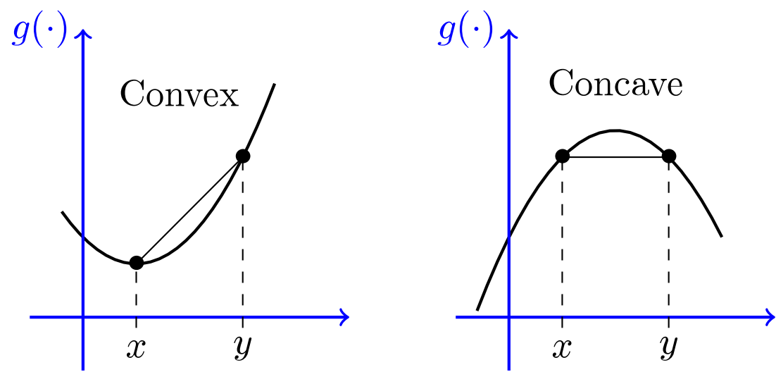
Fig. Pictorial representation of a convex function and a concave function.4
Convex function and concave function
Actually, the definitions of “convex function” and “concave function” etc. are also based on the Jensen’s inequality5:
- The function $f$ is called convex if and only if for all $0<t<1$ and all $x_1,x_2\in X$ such that $x_1\neq x_2$:
- The function $f$ is called strictly convex if and only if for all $0<t<1$ and all $x_1,x_2\in X$ such that $x_1\neq x_2$:
- The function $f$ is said to be concave (resp. strictly concave) if $-f$ is convex (resp. strictly convex).
By the way, there is another practical method to determine if a function $f$ is convex4:
A twice-differentiable function $f\text{: }I\rightarrow\mathbb{R}$ is convex if and only if $f^{\prime\prime}(x)\ge0$ for all $x\in I$.
There are two points should be specially mentioned:
(1) Strictly speaking, the domain of function $f$, $X$, also sometimes denoted as $\mathscr{D}(f)$, should be a convex set6, to technically guarantee that $f\big(\theta x_1+(1-\theta)x_2\big)$ is well defined.3
(2) Although the notations (e.g. $x_1$ and $x_2$) and figures we used above make the input variables of the function $f$ look like scalars in $\mathbb{R}$ (which helps us better understand those notions), they actually refer to $n$-dimensional vectors more commonly, and the function $f$ is defined $\mathbb{R}^n\rightarrow\mathbb{R}$. Correspondingly, the above necessary and sufficient condition, i.e. $f$ is convex iff. $f^{\prime\prime}(x)\ge0$ for all $x\in I$, can be expressed more reasonably, which will be discussed in the later section of this post. See Eq. $\eqref{eq3}$.
Non-convex function
In addition to “convex function” and “concave function”, there is another commonly used term, “non-convex function”, where “non-convex” literally means “not convex”:
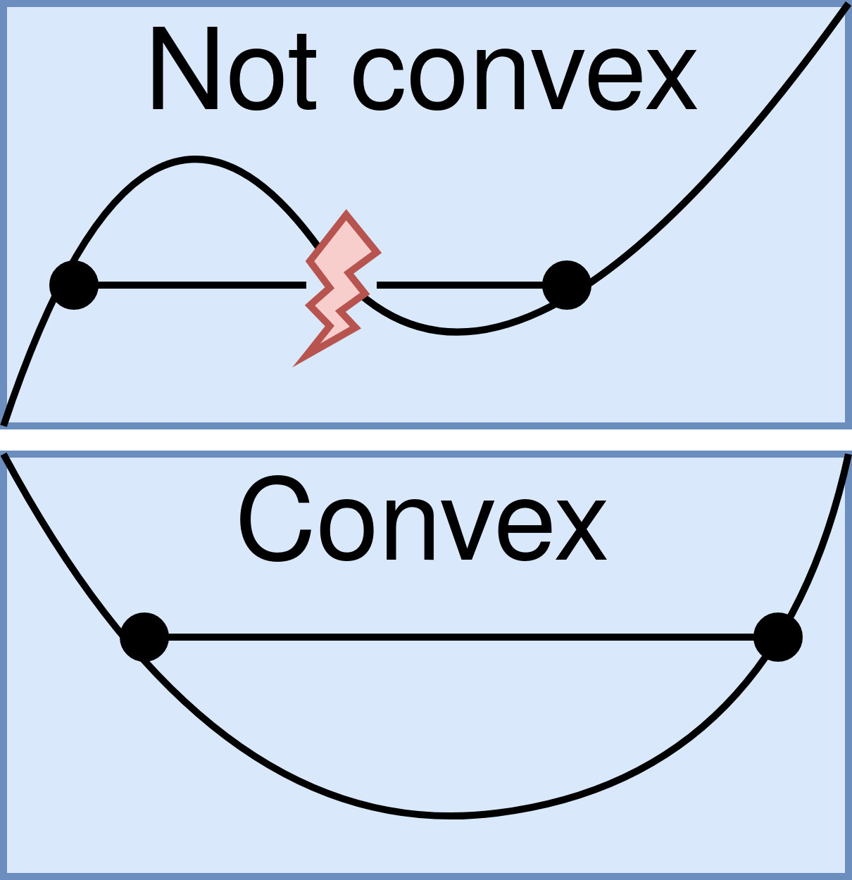
Fig. Convex vs. Not convex.7
A non-convex function can be concave, but it seem that this therm more frequently refers to those functions neither convex nor concave, i.e. there is no a certain relation between $tf(x_1)+(1-t)f(x_2)$ and $f(tx_1+(1-t)x_2)$ for all $x_1$ and $x_2$ in the range.
One of the most significant differences between convex and non-convex functions is that, the convex function has only one global minimum, while non-convex function has both local minima and global minima8:
When selecting an optimization algorithm, it is essential to consider whether the loss function is convex or non-convex. A convex loss function has only one global minimum and no local minima, making it easier to solve with a simpler optimization algorithm. However, a non-convex loss function has both local and global minima and requires an advanced optimization algorithm to find the global minimum.
…
Convex functions are particularly important because they have a unique global minimum. This means that if we want to optimize a convex function, we can be sure that we will always find the best solution by searching for the minimum value of the function. This makes optimization easier and more reliable.
…
A function is said to be non-convex if it is not convex. Geometrically, a non-convex function is one that curves downwards or has multiple peaks and valleys. Looks something like this:
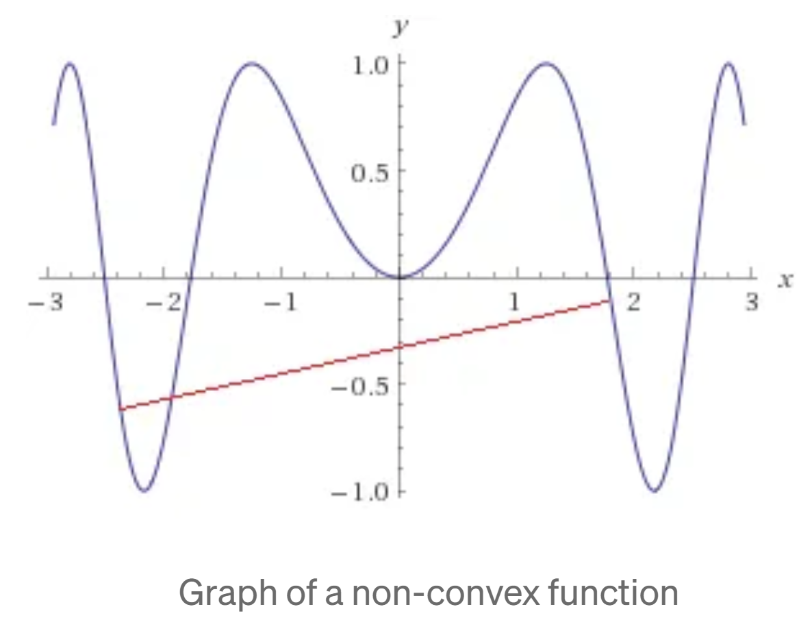
The challenge with non-convex functions is that they can have multiple local minima, which are points where the function has a lower value than all neighboring points.
This means that if we try to optimize a non-convex function, we may get stuck in a local minimum and miss the global minimum, which is the optimal solution we are looking for.
Conditions for convexity and some example of convex functions
First order condition for convexity
The first order condition for convexity is3:
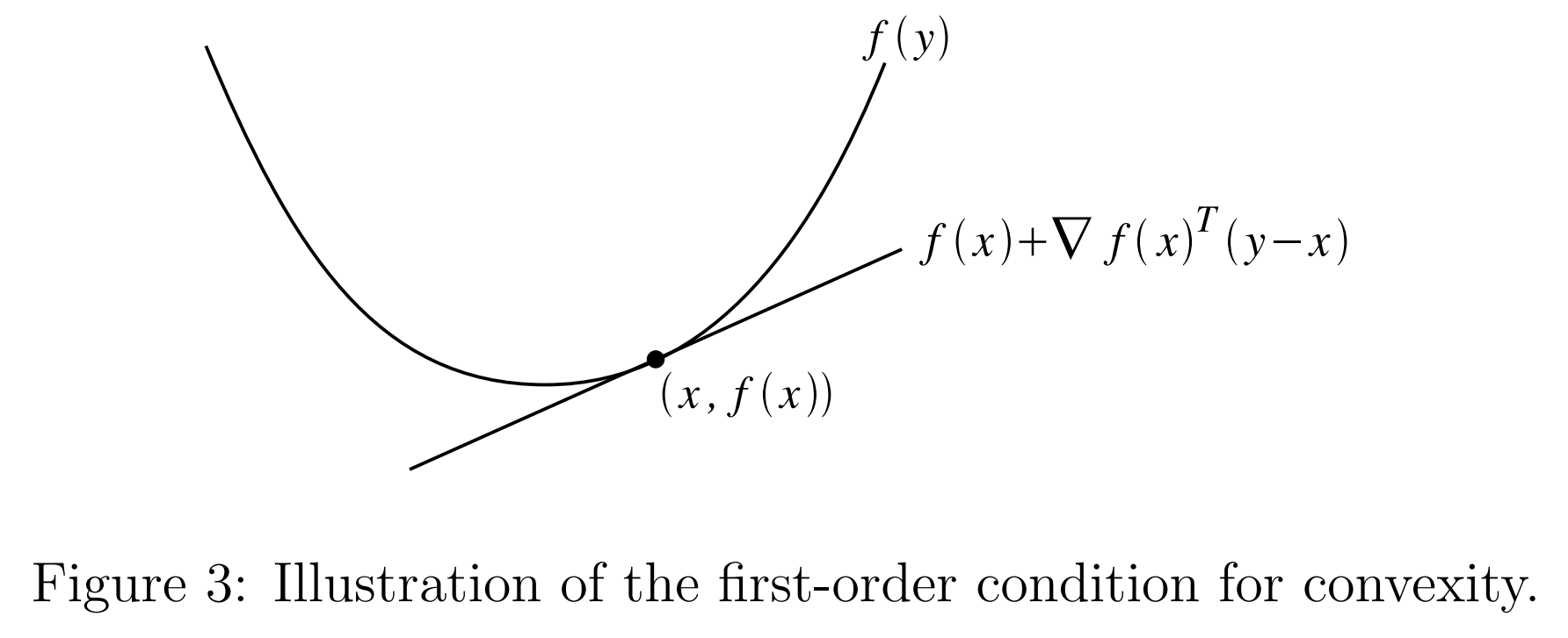
Suppose a function $f:\mathbb{R}^n\rightarrow\mathbb{R}$ is differentiable (i.e., the gradient9 $\nabla_\boldsymbol{\mathrm{x}}f(\boldsymbol{\mathrm{x}})$ exists at all points $\boldsymbol{\mathrm{x}}$ in the domain of $f$). Then $f$ is convex if and only if $\mathscr{D}(f)$ is a convex set and for all $\boldsymbol{\mathrm{x}},\boldsymbol{\mathrm{y}}\in\mathscr{D}(f)$,
\[f(\boldsymbol{\mathrm{y}})\ge f(\boldsymbol{\mathrm{x}})+\nabla_\boldsymbol{\mathrm{x}}f(\boldsymbol{\mathrm{x}})^T(\boldsymbol{\mathrm{y}}-\boldsymbol{\mathrm{x}})\notag\]The function \(f(\boldsymbol{\mathrm{x}})+\nabla_\boldsymbol{\mathrm{x}}f(\boldsymbol{\mathrm{x}})^T(\boldsymbol{\mathrm{y}}-\boldsymbol{\mathrm{x}})\) is also called the first-order approximation to the function $f$ at the point $\boldsymbol{\mathrm{x}}$. Intuitively, this can be thought of as approximating $f$ with its tangent line at the point $\boldsymbol{\mathrm{x}}$. The first order condition for convexity says that $f$ is convex if and only if the tangent line is a global underestimator of the function $f$. In other words, if we take our function and draw a tangent line at any point, then every point on this line will lie below the corresponding point on $f$.
Similar to the definition of convexity, $f$ will be strictly convex if this holds with strict inequality, concave if the inequality is reversed, and strictly concave if the reverse inequality is strict.
Second order condition for convexity
The second order condition for convexity is3:
Suppose a function $f:\mathbb{R}^n\rightarrow\mathbb{R}$ is twice differentiable (i.e., the Hessian9 $\nabla_{\boldsymbol{\mathrm{x}}}^2f(\boldsymbol{\mathrm{x}})$ is defined for all points $\boldsymbol{\mathrm{x}}$ in the domain of $f$). Then $f$ is convex if and only if $\mathscr{D}(f)$ is a convex set and its Hessian is positive semidefinite: i.e., for any $\boldsymbol{\mathrm{x}}\in\mathscr{D}(f)$,3
\[\nabla_{\boldsymbol{\mathrm{x}}}^2f(\boldsymbol{\mathrm{x}})\succeq0.\label{eq3}\]Here, the notation ‘$\succeq$’ when used in conjunction with matrices refers to positive semidefiniteness, rather than componentwise inequality610.11 In one dimension, this is equivalent to the condition that the second derivative $f^{\prime\prime}(x)$ always be positive (i.e., the function always has positive curvature).
Again analogous to both the definition and first order conditions for convexity, $f$ is strictly convex if its Hessian is positive definite, concave if the Hessian is negative semidefinite, and strictly concave if the Hessian is negative definite.
Examples of convex functions
Here are some example of convex functions3.
(1) Exponential functions
Let $f:\mathbb{R}\rightarrow\mathbb{R}$, $f(x)=\mathrm{e}^{ax}$ for any $a\in\mathbb{R}$. Because
\[f^{\prime\prime}(x)=a^2\mathrm{e}^{ax}\ge0\quad\text{for }x\in\mathbb{R}\notag\]and according to $\eqref{eq3}$, exponential functions $f(x)$ are convex.
(2) Negative logarithm
Let $f:\mathbb{R}\rightarrow\mathbb{R}$, $f(x)=-\log x$ with domain \(\mathscr{D}(f)=\mathbb{R}_{++}\), where \(\mathbb{R}_{++}\) denotes the set of strictly positive real numbers. So we have
\[f^{\prime\prime} = \dfrac1{x^2}>0\quad\text{for }x\in\mathbb{R}_{++}\notag\](3) Affine functions
Let $f:\mathbb{R}^n\rightarrow\mathbb{R}$, $f(\boldsymbol{\mathrm{x}})=\boldsymbol{\mathrm{b}}^T\boldsymbol{\mathrm{x}}+c$, where $\boldsymbol{\mathrm{b}}\in\mathbb{R}^n$ and $c\in\mathbb{R}$. For this case, the Hessian matrix is:
\[\nabla_{\boldsymbol{\mathrm{x}}}^2f(\boldsymbol{\mathrm{x}})=\boldsymbol{0}\quad\text{for }\boldsymbol{\mathrm{x}}\in\mathbb{R}^n\notag\]The zero matrix $\boldsymbol{0}$ is both positive semidefinite and negative semidefinite, so $f$ is both convex and concave. It’s easily to understand. For example, intuitively speaking, a one-dimensional affine function
\[f(x) = bx+c\notag\]corresponds a line, and a two-dimensional affine function
\[f(x_1,x_2) = b_1x_1+b_2x_2+c\notag\]corresponds to a plane. In fact, affine functions of this form are the ONLY functions that are both convex and concave.
(4) Quadratic functions
Let $f:\mathbb{R}^n\rightarrow\mathbb{R}$, $f(\boldsymbol{\mathrm{x}})=\frac12\boldsymbol{\mathrm{x}}^T\boldsymbol{\mathrm{A}}\boldsymbol{\mathrm{x}}+\boldsymbol{\mathrm{b}}^T\boldsymbol{\mathrm{x}}+c$, where $\boldsymbol{\mathrm{A}}\in\mathbb{S}^n$, $\boldsymbol{\mathrm{b}}\in\mathbb{R}^n$ and $c\in\mathbb{R}$. The Hessian matrix for the quadratic functions is9:
\[\nabla_{\boldsymbol{\mathrm{x}}}^2f(\boldsymbol{\mathrm{x}})=\boldsymbol{\mathrm{A}}\notag\]Therefore, if the symmetric matrix $\boldsymbol{\mathrm{A}}$ is positive semidefinite (resp. negative semidefinite, positive definite, and negative definite), then the quadratic function is convex (resp. concave, strictly convex, and strictly concave). And, if $\boldsymbol{\mathrm{A}}$ is indefinite then $f$ is neither convex nor concave.
Here is a very classic quadratic function, the squared Euclidean:
\[f(\boldsymbol{\mathrm{x}})=\vert\vert\boldsymbol{\mathrm{x}}\vert\vert_2^2=\boldsymbol{\mathrm{x}}^T\boldsymbol{\mathrm{x}}\notag\]where $\boldsymbol{\mathrm{A}}$ is an identity matrix, and hence the function is a strictly convex function.
(5) Norms
Let $f:\mathbb{R}^n\rightarrow\mathbb{R}$ be some norm on $\mathbb{R}^n$. According to the properties “triangle inequality” and “absolute homogeneity” of the norm, we have:
\[f(\theta\boldsymbol{\mathrm{x}}+(1-\theta)\boldsymbol{\mathrm{y}})\le f(\theta\boldsymbol{\mathrm{x}})+f((1-\theta)\boldsymbol{\mathrm{y}})=\theta f(\boldsymbol{\mathrm{x}})+(1-\theta)f(\boldsymbol{\mathrm{y}})\notag\]Therefore we can conclude that, norms are all convex functions.
It should highlight that, here the convexity of norms is proved by the definition of convex function, rather than by the first order condition or second order condition. The reason is that norms aren’t always differentiable everywhere in the domain $\mathscr{D}(f)$, for example, the $1$-norm
\[\vert\vert\boldsymbol{\mathrm{x}}\vert\vert_1=\sum_{i=1}^n\vert x_i\vert\notag\]is non-differentiable at all points where any $x_i$ is equal to zero.
(6) Nonnegative weighted sums of convex functions
Let $f_1,f_2,\cdots,f_k$ be convex functions and $w_1,w_2,\cdots,w_k$ be nonnegative real numbers, then the function
\[f(\boldsymbol{\mathrm{x}})=\sum_{i=1}^kw_if_i(\boldsymbol{\mathrm{x}})\notag\]is convex, because
\[\begin{split} f(\theta\boldsymbol{\mathrm{x}}+(1-\theta)\boldsymbol{\mathrm{y}}) &=\sum_{i=1}^kw_if_i(\theta\boldsymbol{\mathrm{x}}+(1-\theta)\boldsymbol{\mathrm{y}})\\ &\le\sum_{i=1}^kw_i\big(\theta f_i(\boldsymbol{\mathrm{x}})+(1-\theta)f_i(\boldsymbol{\mathrm{y}})\big)\\ &=\theta\sum_{i=1}^kw_if_i(\boldsymbol{\mathrm{x}})+(1-\theta)\sum_{i=1}^kw_if_i(\boldsymbol{\mathrm{y}})\\ &=\theta f(\boldsymbol{\mathrm{x}})+(1-\theta)f(\boldsymbol{\mathrm{y}}) \end{split}\notag\]References
-
Review Notes and Supplementary Notes CS229 Course Machine Learning Standford University, Convex Optimization Overview, pp. 3-7. ˄ ˄2 ˄3 ˄4 ˄5 ˄6
-
Convex vs. Non-Convex Functions: Why it Matters in Optimization for Machine Learning. ˄
-
LaTeX Component-wise Inequality Symbols: $\preceq$ and $\succeq$ etc. ˄
-
“Similarly, for a symmetric matrix $\boldsymbol{\mathrm{X}}\in\mathbb{S}^n$, $\boldsymbol{\mathrm{X}}\preceq0$ denotes that $\boldsymbol{\mathrm{X}}$ is negative semidefinite. As with vector inequalities, ‘$\le$’ and ‘$\ge$’ are sometimes used in place of ‘$\preceq$’ and ‘$\succeq$’. Despite their notational similarity to vector inequalities, these concepts are very different; in particular, $\boldsymbol{\mathrm{X}}\succeq0$ does not imply that $X_{ij}\ge0$ for all $i$ and $j$.” ˄