Create Animation in MATLAB: Render .gif and .avi File
Introduction
In the previous Blogs, I ever used MATLAB to create .gif file, like animating Bézier curve 1, phase trajectories of Van del Pol Circuit 2 and Chua’s circuit 3. It is a better way to show a changing progress through .gif file rather than static image, but according to my ever experience, MATLAB seems not good at creating GIF, and the worst problem is that it will spend a lot of time for rendering. For example, I use the following script to plot the dynamic solutions of Chua’s circuit in 3 :
1
2
3
4
5
6
7
8
9
10
11
12
13
14
15
16
17
18
19
20
21
22
23
24
25
26
27
28
29
30
31
32
33
34
35
36
37
38
39
40
41
clc,clear,close all

tic
gifFile = "Chua1.gif";
if exist(gifFile,"file")
    delete(gifFile)
end

figure, axes, view(-6.9,37.1)
hold(gca,"on"),box(gca,"on"),grid(gca,"on")
xlabel("x"),ylabel("y"),zlabel("z")
axis([-3,3,-0.4,0.4,-4,4])
h = animatedline(gca,"LineWidth",1.3);

[t,y] = ode45(@chua,[0 100],[0.7 0 0]);

for i = 1:numel(y(:,1))
    addpoints(h,y(i,1),y(i,2),y(i,3))
    drawnow
    exportgraphics(gcf,gifFile,"Append",true);
end
toc

function out = chua(t,in)
x = in(1);
y = in(2);
z = in(3);

alpha  = 15.6;
beta   = 28;
m0     = -1.143;
m1     = -0.714;

h = m1*x+0.5*(m0-m1)*(abs(x+1)-abs(x-1));

xdot = alpha*(y-x-h);
ydot = x-y+z;
zdot  = -beta*y;

out = [xdot,ydot,zdot]';
end
It will create a 71,387 KB .gif file, and the result is fine, but this progress will cost 289.32 seconds, which is too long. So, at that time, I supposed that this is an inherent problem of MATLAB software itself, so I ever tried to learn Python manim package 45, but I didn’t persist since I have no much extra time to do it.
In Script 1, rendering .gif file is realized by appending each figure frame to a .gif file by exportgraphic function with "append" property true. This approach is obtained from official documentation of exportgraphic function 6:
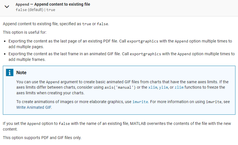
Today, I hear about an interesting officially-held contest “MATLAB Flipbook mini Hack” 7. In this small contest, users could upload their code, that is a user-defined drawframe function 8 which is used to generate a frame of animation, therefore rendering an animation clip. I don’t find out the main function used for invoking drawframe on the official website, but I find a blog of slandarer 9, providing a contestAnimation function to create .gif file:
1
2
3
4
5
6
7
8
9
10
11
12
13
14
15
16
17
18
19
20
21
function contestAnimator()
    animFilename = 'animation.gif'; % Output file name
    firstFrame = true;
    framesPerSecond = 24;
    delayTime = 1/framesPerSecond;
    % Create the gif
    for frame = 1:48
        drawframe(frame)
        fig = gcf();
        fig.Units = 'pixels';
        fig.Position(3:4) = [300,300];
        im = getframe(fig);
        [A,map] = rgb2ind(im.cdata,256);
        if firstFrame
            firstFrame = false;
            imwrite(A,map,animFilename, LoopCount=Inf, DelayTime=delayTime);
        else
            imwrite(A,map,animFilename, WriteMode="append", DelayTime=delayTime);
        end
    end
end
Luckily, it works. Script 2 gets each frame using getframe function and post-process it by rgb2ind function, and finally appends frame to .gif file by imwrite function. And in fact, it is similar to the way of generating .gif file provided by imwrite official documentation 10:
1
2
3
4
5
6
7
8
9
10
...
filename = "testAnimated.gif"; % Specify the output file name
for idx = 1:nImages
    [A,map] = rgb2ind(im{idx},256);
    if idx == 1
        imwrite(A,map,filename,"gif","LoopCount",Inf,"DelayTime",1);
    else
        imwrite(A,map,filename,"gif","WriteMode","append","DelayTime",1);
    end
end
So, in the following text, I will make a detailed analysis for getframe, rgb2ind and imwrite functions in Script 2, and afterward, apply this method to rendering dynamic solutions of Chua’s circuit, and compare it with Script 1. Finally, a similar way of creating .avi video file is provided.
getframe function
MATLAB getframe function 11 is used to “Capture axes or figure as movie frame”. The basic usage of it is:
1
2
3
4
5
6
7
8
9
10
11
rng("default")
x = rand(1,4);
y = rand(1,4);
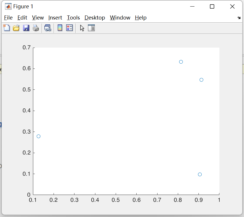
scatter(x,y)
fig = gcf();
ax = gca();
% Capture axes as movie frame
F1 = getframe(ax)
% Capture figure as movie frame
F2 = getframe(fig)
where the figure will show like this:
and both F1 and F2 are struct variables:
1
2
3
4
5
6
7
8
9
F1 =
  struct with fields:
       cdata: [514×652×3 uint8]
    colormap: []

F2 =
  struct with fields:
       cdata: [630×840×3 uint8]
    colormap: []
and whose cdata fields are RGB-tuples:
1
2
3
4
5
6
7
8
9
10
11
12
13
14
15
16
17
>> F1.cdata(1,1,:), F2.cdata(1,1,:)

  1×1×3 uint8 array
ans(:,:,1) =
   240
ans(:,:,2) =
   240
ans(:,:,3) =
   240

  1×1×3 uint8 array
ans(:,:,1) =
   240
ans(:,:,2) =
   240
ans(:,:,3) =
   240
We could reproduce axes or figure using imshow function:
1
2
figure("Color",[7,84,213]/255)
imshow(F1.cdata)
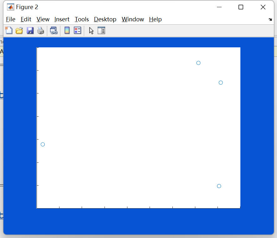
1
2
figure("Color",[7,84,213]/255)
imshow(F2.cdata)
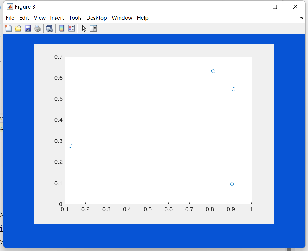
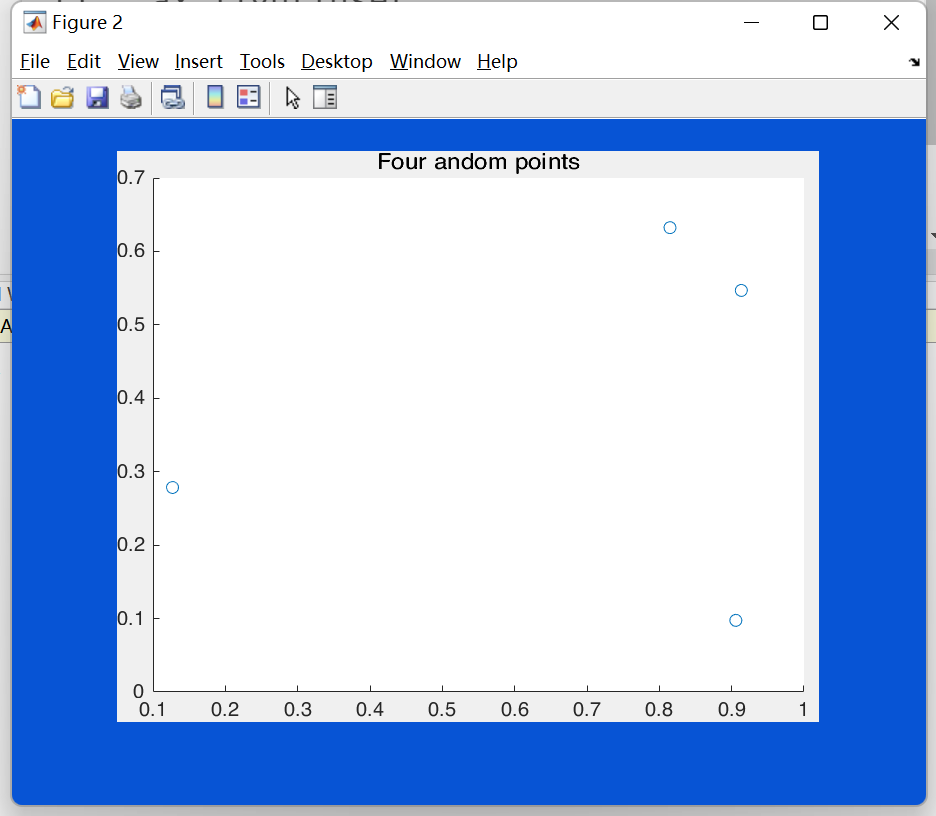
The difference of capturing axes and capturing figure is clear to see. And what’s more, we could specify the second input argument, which is a four-element array, to get the specified area, like “Calculate Region to Include Title and Labels” example obtained from official documentation 11:
1
2
3
4
5
6
7
8
9
10
11
12
13
14
15
16
17
18
clc,clear,close all

rng("default")
x = rand(1,4);
y = rand(1,4);
scatter(x,y)
title("Four andom points")

ax = gca();
ax.Units = "pixels";
pos = ax.Position;
ti = ax.TightInset;

rect = [-ti(1), -ti(2), pos(3)+ti(1)+ti(3), pos(4)+ti(2)+ti(4)];
F = getframe(ax,rect);

figure("Color",[7,84,213]/255)
imshow(F.cdata)
rgb2ind function
After getting a frame, we could save it using imwrite function 12, by (1) saving RGB image, or by (2) saving indexed image. The second way relies on using rgb2ind function 13 to convert RGB image to indexed image. For example:
1
2
3
4
5
6
7
8
9
10
11
12
13
14
15
16
17
18
clc,clear,close all

rng("default")
x = rand(1,4);
y = rand(1,4);
scatter(x,y)
fig = gcf();
ax = gca();

% Capture axes as movie frame
F = getframe(ax);

% Save figure by RGB image
imwrite(F.cdata,"jpg-1.jpg");

% Save figure by indexed image
[A,map] = rgb2ind(F.cdata,256);
imwrite(A,map,"jpg-2.jpg")
and the jpg-1.jpg and jpg-2.jpg is exactly the same:
1
2
3
4
5
clc,clear,close all

a = imread("jpg-1.jpg");
b = imread("jpg-2.jpg");
whos
1
2
3
 Name        Size                 Bytes  Class    Attributes
  a         514x652x3            1005384  uint8
  b         514x652x3            1005384  uint8
1
2
3
>> sum(a-b,"all")
ans =
     0
So, I speculate that, at this case, if the input of imwrite function is indexed image and whose map, imwrite function will convert it to RGB image automatically.
However, if we want to use imwrite to save RGB image to a .gif file, it will throw an error:
1
2
3
4
5
6
7
8
9
10
11
12
13
14
clc,clear,close all

rng("default")
x = rand(1,4);
y = rand(1,4);
scatter(x,y)
fig = gcf();
ax = gca();

% Capture axes as movie frame
F = getframe(ax);

% Save figure by RGB-tuple
imwrite(F.cdata,"gif.gif",WriteMode="append");
1
2
3
4
5
6
7
8
9
Error using writegif
3-D data not supported for GIF files. Data
must be 2-D or 4-D.

Error in imwrite (line 566)
        feval(fmt_s.write, data, map, filename, paramPairs{:});

Error in script6 (line 14)
imwrite(F.cdata,"gif.gif",WriteMode="append");
So, it explains why Script 2 adopts the second way, that is saving indexed image by imwrite function, rather than RGB image. (imwrite document 10 mentions this point as well.)
The outputs of code in Script 3:
1
[A,map] = rgb2ind(F.cdata,256);
A is indexed image, and map is the associated colormap.
Specifically, each row of map is a RGB-tuple, representing a specific color, and the number of colors is determined by the second input argument “Number of quantized colors” Q (here is 256) or “Tolerance used for uniform quantization” tol (concerning quantization algorithm 14). As for A, if the size of F.cdata is $h\times w\times 3$, then the size of A is $h \times w$, and each element $e_{i,j}$ in A denotes an index corresponding to the color order in map.
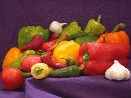
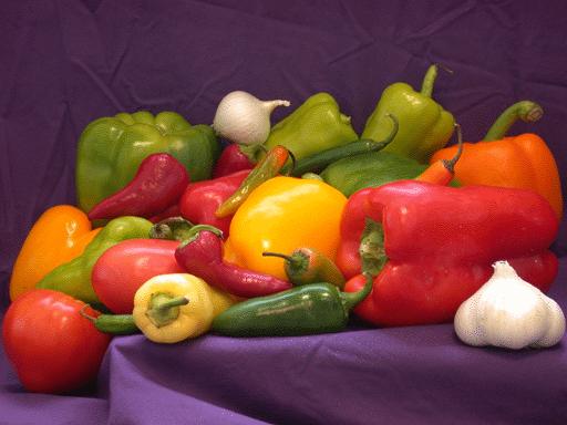
For example, I found a colorful image “pepper.png” downloaded with MATLAB:
1
2
3
4
5
6
7
clc,clear,close all

img = imread("peppers.png");
imshow(img)
F = getframe(gca());

[A,map] = rgb2ind(F.cdata,256);
N.B., If we choose a more colorful image, the number of colors in map is determined by “Number of quantized colors” Q more, otherwise, it will mainly determined by “Tolerance used for uniform quantization” tol. And at the latter case, it is more less than the Q we specified.
For A and map at this case:
1
2
3
4
5
6
7
>> size(F.cdata), size(A), size(map)
ans =
   384   512     3
ans =
   384   512
ans =
   256     3
1
2
3
4
5
6
7
8
>> F.cdata(2,1,:)
  1×1×3 uint8 array
ans(:,:,1) =
   63
ans(:,:,2) =
   31
ans(:,:,3) =
   62
1
2
3
>> map(A(2,1)+1,:)*255
ans =
    59    29    59
N.B., Here, we add one to each element in A to find a corresponding color in map. This detail is obtained from 15, “If the image matrix is of data type logical, uint8 or uint16, the colormap normally contains integer values in the range $[0, p–1]$ (where $p$ is the length of the colormap). The value 0 points to the first row in the colormap, the value 1 points to the second row, and so on.”
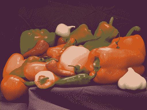
As can be seen, the RGB-tuple found based on A and map, (59,29,59), is very similar to that original RGB array in F.cdata, (63,31,62). However, they are not exactly the same, so in this image conversion process, some color information is lost. If we decrease the Q value further, this kind of distortion becomes more serious:
1
2
3
4
5
6
7
8
9
10
11
12
13
clc,clear,close all

img = imread("peppers.png");
imshow(img)
F = getframe(gca());

[A1,map1] = rgb2ind(F.cdata,4);
[A2,map2] = rgb2ind(F.cdata,50);
[A3,map3] = rgb2ind(F.cdata,256);

imwrite(A1,map1,"img-1.jpg")
imwrite(A2,map2,"img-2.jpg")
imwrite(A3,map3,"img-3.jpg")
The original and the three saved figures show as follows:

The maximum value of Q is $65,536$ 13:
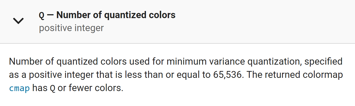
However, in Script 4, specifying Q as the value over $256$ will cause some problems.
If we use the following code, which is similar to Script 4, to convert and save image:
1
2
[A4,map4] = rgb2ind(F.cdata,65536);
imwrite(A4,map4,"img-4.jpg")
imwrite function will throw an error while saving:
1
2
3
4
5
6
7
8
9
10
11
Error using writejpg>set_jpeg_props
UINT16 image data requires bitdepth specifically set to either 12 or 16.

Error in writejpg (line 49)
props = set_jpeg_props(data,varargin{:});

Error in imwrite (line 566)
        feval(fmt_s.write, data, map, filename, paramPairs{:});

Error in script5 (line 16)
imwrite(A4,map4,"img-4.jpg")
It reminds us to specify a higher value for "BitDepth" property, i.e.,
1
2
[A4,map4] = rgb2ind(F.cdata,65536);
imwrite(A4,map4,"img-4.jpg","BitDepth",16)
It works and without any error, however, image img-4.jpg can’t inspected in Windows image viewer:
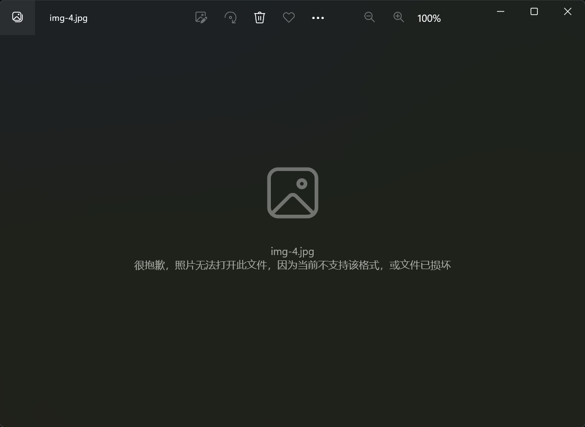
I suppose that Windows image viewer doesn’t support viewing the image with this kind of bit depth.
But on another hand, we could import this unit16 image using imread function, and view it by imshow function:
1
2
3
4
clc,clear,close all

img = imread("img-4.jpg");
imshow(img)
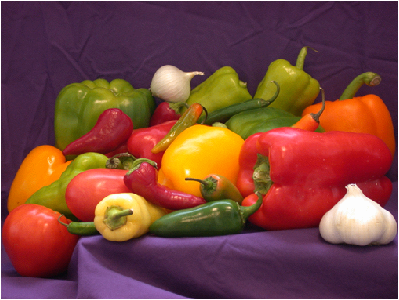
1
2
3
>> class(img)
ans =
    'uint16'
More detailed information about indexed image could be found in 13 and 15.
imwrite function
As described above, imwrite function 12 is used to append multiple indexed images to an identical .gif file, and specifically, the corresponding code in Script 2 is:
1
2
3
4
5
6
7
8
9
10
11
12
13
...
	firstFrame = true;
	...
    for frame = 1:48
        ...
        if firstFrame
            firstFrame = false;
            imwrite(A,map,animFilename,LoopCount=Inf,DelayTime=delayTime);
        else
            imwrite(A,map,animFilename,WriteMode="append",DelayTime=delayTime);
        end
    end
...
When saving the first fame, two properties of imwrite function, LoopCount and DelayTime, are specified, and when appending the subsequence frames, WriteMode and DelayTime are used. The meaning of specifying WriteMode as "append" is clear, so here we just need to understand what LoopCount and DelayTime are.
(1) LoopCount is the number of times to repeat the animation, and a LoopCount value of Inf causes the animation to loop continuously 12:
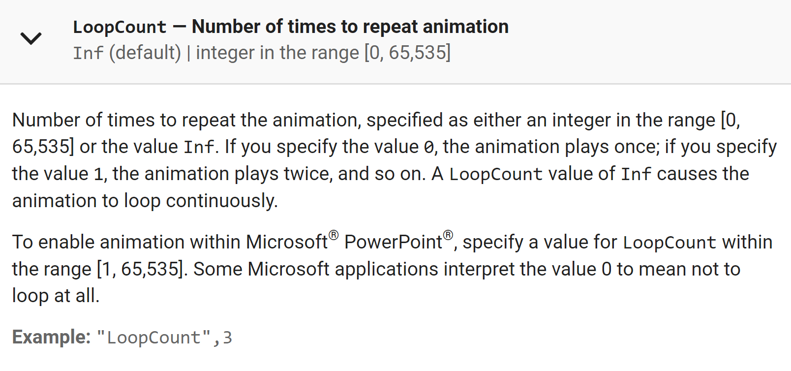
For example, if we specify it as 1, the generated .gif will stop repeating after animating $1$ times. We just need to set this property when creating the first frame.
(2) DelayTime is the delay before displaying next image (frame) 12:
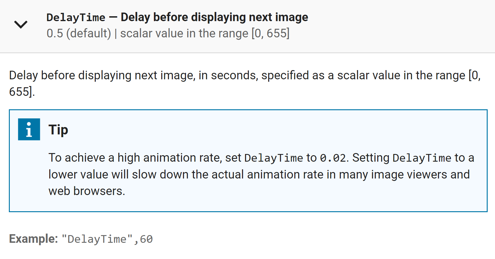
Actually, it is the reciprocal of FPS (Frames Per Second, i.e., frame rate). The small tip in the documentation (the above figure) should be noted, “Setting DelayTime to a lower value will slow down the actual animation rate in many image viewers and web browsers.” This point will be discussed in the following section.
Render .gif file by imwrite function
After learning about details in Script 2, we could modify Script 1, which is used to generate a .gif file showing dynamic solutions of Chua’s circuit, to the following code:
1
2
3
4
5
6
7
8
9
10
11
12
13
14
15
16
17
18
19
20
21
22
23
24
25
26
27
28
29
30
31
32
33
34
35
36
37
38
39
40
41
42
43
44
45
46
47
48
49
50
51
52
53
54
55
56
clc,clear,close all

tic
figure("Color","w")
axes
view(-6.9,37.1)
hold(gca,"on"),box(gca,"on"),grid(gca,"on")
xlabel("x"),ylabel("y"),zlabel("z")
axis([-3,3,-0.4,0.4,-4,4])
h = animatedline(gca,"LineWidth",1.3);

firstFrame = true;
framesPerSecond = 24;
delayTime = 1/framesPerSecond;

gifFile = sprintf("Chua%s.gif",num2str(framesPerSecond));
if exist(gifFile,"file")
    delete(gifFile)
end

[t,y] = ode45(@chua,[0 100],[0.7 0 0]);

for i = 1:numel(y(:,1))
    addpoints(h,y(i,1),y(i,2),y(i,3))

    fig = gcf();
    im = getframe(fig);
    [A,map] = rgb2ind(im.cdata,256);

    if firstFrame
        firstFrame = false;
        imwrite(A,map,gifFile,LoopCount=Inf,DelayTime=delayTime);
    else
        imwrite(A,map,gifFile,WriteMode="append",DelayTime=delayTime);
    end
end
toc

function out = chua(t,in)
x = in(1);
y = in(2);
z = in(3);

alpha  = 15.6;
beta   = 28;
m0     = -1.143;
m1     = -0.714;

h = m1*x+0.5*(m0-m1)*(abs(x+1)-abs(x-1));

xdot = alpha*(y-x-h);
ydot = x-y+z;
zdot  = -beta*y;

out = [xdot,ydot,zdot]';
end
It will generate a 24-fps .gif file, showing below:

the generation process spends 55.35 seconds, and the file size is 69,244 KB.
As can be seen, compared with Script 1, using Script 5 to generate .gif file makes rendering time reduce from 289.32 seconds to 55.35 seconds, which is a great improvement.
What’s more, in Script 5, the PFS of .gif file (and hence animation speed) could be adjusted, while in Script 1 it is not possible, cause exportgraphics function 6 doesn’t provide a similar property like DelayTime of imwrite function.
If we change framesPerSecond in Script 5 from 24 to 60, and 200, respectively (that is changing DelayTime from 1/24, to 1/60, and 1/200), the generated .gif file show as follows:


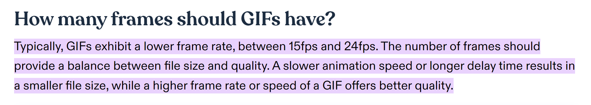
The results show that, (1) basically, changing DelayTime doesn’t influence the script rendering time and .gif file size, and (2) decreasing DelayTime indeed could increase the animation speed, but as mentioned above, specifying too small DelayTime value will slow down the speed instead.
Actually, the second item is commonsensible, because .gif format itself isn’t designed for presenting high-FPS animation, and commonly, the FPS of a .gif file is between 15 and 24 16:
If we want to present high frame rate, video file is a better choice, and some concerned content will be discussed in the next section.
On another hand, if we maximize the .gif in the viewer, we could find that its resolution is kinda low. To improve this point, we could change the Position property at the beginning when creating the figure:
1
2
3
4
5
...
figure("Color","w")
fig = gcf();
fig.Position(3:4) = [1920,1080];
...
it will increase the resolution of .gif file, but meanwhile, rendering time will significantly level up to 304.08 seconds, and file size will also increase to 278 MB.
Render .avi video file
Using .gif file to present animation is very convenient when sharing contents on the Internet, as it could be stored in image hosting service, and others could get access to it through external link. But as described in the above section, the FPS of .gif file is limited when using imwrite function. Therefore, if we want to increase the frame rate further and don’t expect to put the animation file in the image hosting service, creating video file is a better approach. In fact, Python manim package 4, which is used to create animation in Python, also supports both options.
In MATLAB, creating video file is similar to creating .gif file, that is frame by frame. But at this case, we should use VideoWriter 17 and writeVideo 18 instead. The complete code for rendering a .avi file shows as follows:
1
2
3
4
5
6
7
8
9
10
11
12
13
14
15
16
17
18
19
20
21
22
23
24
25
26
27
28
29
30
31
32
33
34
35
36
37
38
39
40
41
42
43
44
45
46
47
48
49
50
51
clc,clear,close all

tic
figure("Color","w")
axes
view(-6.9,37.1)
hold(gca,"on"),box(gca,"on"),grid(gca,"on")
xlabel("x"),ylabel("y"),zlabel("z")
axis([-3,3,-0.4,0.4,-4,4])
h = animatedline(gca,"LineWidth",1.3);

FrameRate = 60;
aviFile = sprintf("Chua%s.avi",num2str(FrameRate));
if exist(aviFile,"file")
    delete(aviFile)
end

v = VideoWriter(aviFile);
v.FrameRate = FrameRate;
open(v)

[t,y] = ode45(@chua,[0 100],[0.7 0 0]);

for i = 1:numel(y(:,1))
    addpoints(h,y(i,1),y(i,2),y(i,3))

    fig = gcf();
    im = getframe(fig);
    writeVideo(v,im);
end
close(v)
toc

function out = chua(t,in)
x = in(1);
y = in(2);
z = in(3);

alpha  = 15.6;
beta   = 28;
m0     = -1.143;
m1     = -0.714;

h = m1*x+0.5*(m0-m1)*(abs(x+1)-abs(x-1));

xdot = alpha*(y-x-h);
ydot = x-y+z;
zdot  = -beta*y;

out = [xdot,ydot,zdot]';
end
Among which, v.FrameRate = FrameRate; is to specify the frame rate, if we change it and increase to a relatively high value, we could find video duration is decreased accordingly:
.avi File |
FrameRate |
Script running time | File size | Video duration |
|---|---|---|---|---|
| 1 | 24 | 31.38 | 118,449 KB | 01 min 35 sec |
| 2 | 60 | 38.73 | 118,449 KB | 38 sec |
| 3 | 120 | 33.90 | 118,449 KB | 19 sec |
| 4 | 200 | 35.05 | 118,449 KB | 11 sec |
Similarly, if we want to increase resolution, we could change the Position property (like we do for .gif file), and change the Quality property of VideoWriter:
1
2
3
4
5
6
7
8
9
10
11
...
figure("Color","w")
fig = gcf();
fig.Position(3:4) = [3840,2160];
...
Quality = 100;
v = VideoWriter(aviFile);
v.FrameRate = FrameRate;
v.Quality = Quality;
open(v)
...
and of course, it will spend a rather long time for rendering, and occupies much more storage space.
What’s more, choosing other video file format of VideoWriter function (default value is "Motion JPEG AVI")17 may help:

but I know less about compression and encoding methods of video file, so here I don’t try this way and make a comparison.
References
-
Bernstein polynomial and Bézier curve - What a starry night~. ˄
-
Nonlinear Oscillation Circuit: Van del Pol Circuit - What a starry night~. ˄
-
Chaotic Circuit, Chua’s Circuit - What a starry night~. ˄ ˄2
-
MATLAB
exportgraphics: Save plot or graphics content to file - MathWorks. ˄ ˄2 -
MATLAB
getframe: Capture axes or figure as movie frame - MathWorks China. ˄ ˄2 -
MATLAB
imwrite: Write image to graphics file - MathWorks. ˄ ˄2 ˄3 ˄4 -
MATLAB
rgb2ind: Convert RGB image to indexed image - MathWorks. ˄ ˄2 ˄3 -
MATLAB
rgb2ind: Tolerance used for uniform quantizationtol- MathWorks China. ˄ -
Image Types in the Toolbox: Indexed Images - MathWorks. ˄ ˄2
-
MATLAB
VideoWriter: Create object to write video files - MathWorks China. ˄ ˄2