Introduction

MATLAB have four built-in functions, confusionmat ¹, confusionchart ², confusion ³, and plotconfusion ⁴, to calculate or visualize confusion matrix for classification problems. These four functions are from “AI, Data Science, and Statistics” topic ⁵: confusionmat and confusionchart are provided by Statistics and Machine Learning Toolbox; confusion and plotconfusion by Deep Learning Toolbox. But, although all of them are about confusion matrix, the outputs of different functions are not exactly the same, which may make users confused. Therefore in this blog, on fisheriris data set, I will train an SVM using training features X_training and corresponding labels Y_training, and use this SVM to predict test features X_test, whose predictions are stored in variable pred. At last, the confusion matrix are computed on pred and real labels Y_test, but confusion matrix computation is realized by different aforementioned built-in functions. By comparing whose outputs in detail, this blog will organize the use of these functions.

confusionmat and confusionchart functions

For confusionmat ¹ and confusionchart ² functions from Statistics and Machine Learning Toolbox:

1
2
3
4
5
6
7
8
9
10
11
12
13
14
15
16
17
18
19
20
21
22
23
24
25
26
27
28
29
clc,clear,close all

% Load dataset
load fisheriris.mat
rng("default")

% Preprocess labels
species = string(species);

% Partition dataset
cv = cvpartition(species,"HoldOut",0.3);
X_training = meas(cv.training,:);
Y_training = species(cv.training,:);
X_test = meas(cv.test,:);
Y_test = species(cv.test,:);

% Construct and train an SVM
mdl = fitcecoc(X_training,Y_training, ...
    "Learners",templateSVM("Standardize",true));

% Test the SVM
pred = string(mdl.predict(X_test));
% It is necessary to convert cell to string array for `confusionchart` function
acc = sum(pred==Y_test)/numel(Y_test);

% Calculate confusion matrix
[cm,order] = confusionmat(Y_test,pred);
% Visualize confusion matrix
cmplot = confusionchart(Y_test,pred);

The outputs of confusionmat function

confusionmat could provides two outputs:

1
2
3
4
5
6
7
8
9
10
11
>> cm,order
cm =
    15     0     0
     0    14     1
     0     0    15
     
order = 
  3×1 string array
    "setosa"
    "versicolor"
    "virginica"

where cm is the specific confusion matrix, and order is a string array (the same data type as input labels) that contains class names.

The outputs of confusionchart function

confusionchart will plot the confusion matrix in the figure:

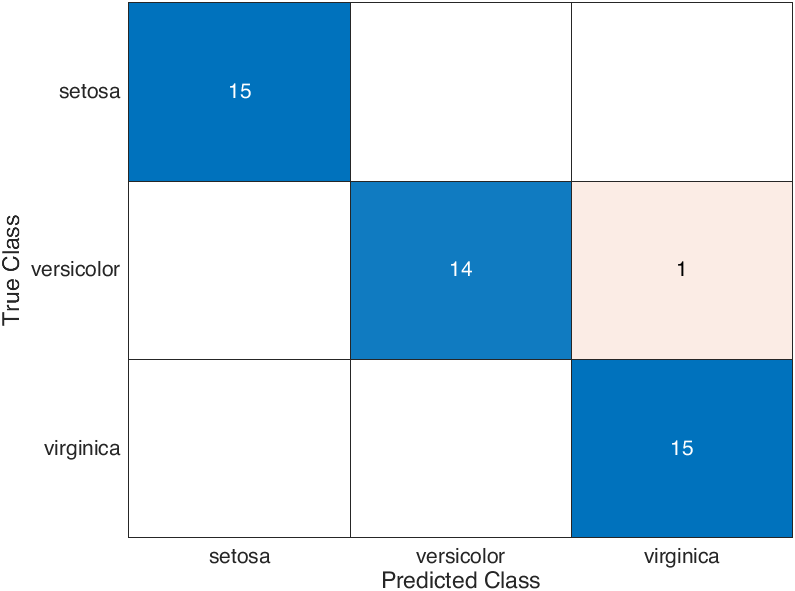
and the data type of its output cmplot is ConfusionMatrixChart, whose properties shows as follows:

1
2
3
4
5
6
7
8
9
10
11
12
13
14
15
16
17
18
19
20
21
22
23
24
25
26
27
28
>> cmplot
cmplot = 
  ConfusionMatrixChart with properties:
    NormalizedValues: [3×3 double]
         ClassLabels: [3×1 string]
           ClassLabels: [3×1 string]
         ColumnSummary: 'off'
         DiagonalColor: [0 0.4471 0.7412]
             FontColor: [0.1500 0.1500 0.1500]
              FontName: 'Helvetica'
              FontSize: 10
           GridVisible: on
      HandleVisibility: 'on'
         InnerPosition: [0.1467 0.1100 0.7583 0.8150]
                Layout: [0×0 matlab.ui.layout.LayoutOptions]
         Normalization: 'absolute'
      NormalizedValues: [3×3 double]
      OffDiagonalColor: [0.8510 0.3255 0.0980]
         OuterPosition: [0 0 1 1]
                Parent: [1×1 Figure]
              Position: [0.1467 0.1100 0.7583 0.8150]
    PositionConstraint: 'outerposition'
            RowSummary: 'off'
                 Title: ''
                 Units: 'normalized'
               Visible: on
                XLabel: 'Predicted Class'
                YLabel: 'True Class'

where NormalizedValues and ClassLabels properties are confusion matrix and class names, respectively:

1
2
3
4
5
6
7
8
9
10
11
>> cmplot.NormalizedValues, cmplot.ClassLabels
ans =
    15     0     0
     0    14     1
     0     0    15

ans = 
  3×1 string array
    "setosa"
    "versicolor"
    "virginica"

confusion and plotconfusion functions

For confusion ³ and plotconfusion ⁴ functions from Deep Learning Toolbox:

1
2
3
4
5
6
7
8
9
10
11
12
13
14
15
16
17
18
19
20
21
22
23
24
25
26
27
28
29
30
31
32
33
34
35
36
37
clc,clear,close all

% Load dataset
load fisheriris.mat
rng("default")

% Preprocess labels
species = string(species);
species_num = nan(size(species));
species_num(species=="setosa") = 1;
species_num(species=="versicolor") = 2;
species_num(species=="virginica") = 3;
species = species_num;

% Partition dataset
cv = cvpartition(species,"HoldOut",0.3);
X_training = meas(cv.training,:);
Y_training = species(cv.training,:);
X_test = meas(cv.test,:);
Y_test = species(cv.test,:);

% Construct and train an SVM
mdl = fitcecoc(X_training,Y_training,"Learners",templateSVM("Standardize",true));

% Test the SVM
pred = mdl.predict(X_test);
acc = sum(pred==Y_test)/numel(Y_test);

% Convert labels to one-hot vector
Y_test = ind2vec(Y_test'); % Transpose is necessary
pred = ind2vec(pred'); % Transpose is necessary

% Calculate confusion matrix
[c,cm,ind,per] = confusion(Y_test,pred);
% Visualize confusion matrix
figure("Color","w")
cmplot = plotconfusion(Y_test,pred);

In oder to use confusion and plotconfusion, two points should be noted here:

(1) The labels specified by strings should be converted to corresponding numeric data, and

(2) the numeric data should be convert to one-hot vector using ind2vec function ⁶.

Note: After converting to one-hot vector, both Y_test and pred are of sparse double data type ⁷:

1
2
3
4
5
6
7
>> Y_test
Y_test =
   (1,1)        1
   (1,2)        1
   (1,3)        1
   (1,4)        1
   ......

1
2
3
4
5
6
pred =
   (1,1)        1
   (1,2)        1
   (1,3)        1
   (1,4)        1
   ......

By the way, we could use full function ⁸ to convert the sparse matrix to full storage.

The outputs of confusion function

The confusion could create four outputs:

1
2
3
4
5
6
7
8
9
10
11
12
13
14
15
16
17
18
19
>> c,cm,ind,per
c =
    0.0222

cm =
    15     0     0
     0    14     1
     0     0    15

ind =
  3×3 cell array
    {[1 2 3 4 5 6 7 8 9 10 … ]}    {1×0 double               }    {1×0 double               }
    {1×0 double               }    {[16 17 18 19 20 21 22 … ]}    {[                     23]}
    {1×0 double               }    {1×0 double               }    {[31 32 33 34 35 36 37 … ]}

per =
         0         0    1.0000    1.0000
    0.0323         0    1.0000    0.9677
         0    0.0625    0.9375    1.0000

where:

(1) c is confusion value, i.e., fraction of misclassified samples, or rather, $1-\mathrm{accuracy}$;

(2) cm is the specific confusion matrix;

(3) ind contains the sample indices of class $i$ target classified as class $j$. For example, for the $23$-th test sample, its prediction by SVM is $3$-th class ("virginica") while whose real label is $2$-th class ("versicolor");

(4) per is a matrix of percentages, where each row summarizes four percentages associated with the $i$-th class, that is:

The outputs of plotconfusion function

As for plotconfusion, it will create an output cmplot, and plot a confusion matrix in the figure:

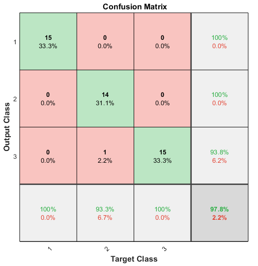
This figure displays more information than that created by confusionchart, but cmplot is MATLAB Figure class, and it seems that we couldn’t obtain the specific confusion matrix from cmplot, which is not convenient if we just use plotconfusion without confusion. What’s more, this confusion matrix plot is kind of weired, because it takes “Target Class” (Actual Condition) as column name, and “Output Class” (Predicted Condition) as row name, making it the transpose of those matrix created by confusionmat, confusionchart, and confusion (like Fig. 1). It is really not common.

Conclusion

In conclusion, I think confusion is the best choice if we want to record confusion matrix for classification problem, despite of the fact that we need to process the label variables in advance.

References