Monte Carlo Simulation to Estimate $\pi$
Recently, I heard about a small official MATLAB contest, “MATLAB Flipbook mini Hack” 1, and in this contest participants should upload a user-defined function for rendering a short animation, that is a .gif file. I feel that many works in the gallery 1 are very amazing, cause participants are just allowed to upload an easy function drawframe(f) (up to 2,000 characters 2), which is for creating a single frame, therefore, the transition between a frame and its subsequent frame is just realized by mathematical operations! Excited by it, I learned a better way to create .gif file in MATLAB (refer to Blog 3). And today I found a Mike’s work 4 animating Monte Carlo estimation for $\pi$. This is a very classical example to illustrate the wisdom of Mote Carlo simulation. Mike’s code 4 is clear and straightforward, but when I want to enrich some details on which, I encountered some problems, so I will record them in this blog. The final .gif file I created shows as follows, and my main improvement is about showing more text information:
the complete code is:
1
2
3
4
5
6
7
8
9
10
11
12
13
14
15
16
17
18
19
20
21
22
23
24
25
26
27
28
29
30
31
32
33
34
35
36
37
38
39
40
41
42
43
44
45
46
47
48
49
50
51
52
53
54
55
56
57
58
59
60
61
62
63
64
65
66
67
68
69
70
71
72
73
74
75
76
77
78
79
80
81
82
83
84
85
86
87
88
clc,clear,close all

rng("default")
gifFileName = "gif.gif";
if exist(gifFileName,"file")
    delete(gifFileName)
end
fps = 24;

figure("Color","w","Position",[1000,918,694.33,420])

tiledlayout(3,3,"TileSpacing","tight")
nexttile(1,[3,2])
ax1 = gca();

nexttile(6)
ax2 = gca();

for f = 1:500
    helperDrawFrame(f,ax1,ax2)
    fig = gcf();
    im = getframe(fig);
    [A,map] = rgb2ind(im.cdata,256);
    if f == 1
        imwrite(A,map,gifFileName,"LoopCount",Inf,"DelayTime",1/fps)
    else
        imwrite(A,map,gifFileName,"WriteMode","append","DelayTime",1/fps)
    end
end


function helperDrawFrame(f,ax1,ax2)
persistent total_points inside_points outside_points
if f == 1
    total_points = 0;
    inside_points = 0;
    outside_points = 0;
end

% Settings for ax1
set(ax1,"Xlim",[-1,1],"YLim",[-1,1], ...
    "FontSize",15,"FontName","Times New Roman", ...
    "LineWidth",1.2)
ax1.Toolbar.Visible = "off";
hold(ax1,"on"),box(ax1,"on")
daspect(ax1,[1,1,1])

% Settings for ax2
set(ax2,"Visible","off")
hold(ax2,"off")

% Carry out Monte Carlo simulation in ax1
pointsPerCount = f*50;
total_points = total_points+pointsPerCount;

x = 2*rand(1,pointsPerCount)-1;
y = 2*rand(1,pointsPerCount)-1;
d = sqrt(x.^2+y.^2);
idx = d<=1;
inside_points = inside_points+sum(idx);
outside_points = outside_points+sum(~idx);

theta = 0:0.01:2*pi;
plot(ax1,cos(theta),sin(theta),"LineWidth",1.5,"Color","k")
scatter(ax1,x(idx),y(idx),1,"b.");
scatter(ax1,x(~idx),y(~idx),1,"r.");

% Display information in ax2
cla(ax2)
estimatedPi = num2str(4*inside_points/total_points,"%.8f");
realPi = '3.14159265';
idx = find(diff(realPi(1:end)==estimatedPi(1:end)) == -1);
idx = idx(1);

FontSize = 15;
vSpace = 0.5;
text(ax2,0,3*vSpace,sprintf("Total points: %s",num2str(total_points)), ...
    "FontSize",FontSize,"FontName","Times New Roman")
text(ax2,0,2*vSpace,sprintf("Inside points: %s",num2str(inside_points)), ...
    "FontSize",FontSize,"FontName","Times New Roman")
text(ax2,0,1*vSpace,sprintf("Outside points: %s",num2str(outside_points)), ...
    "FontSize",FontSize,"FontName","Times New Roman")
text(ax2,0,0,sprintf("Real %s: %s%s%s%s...","\pi","\color{blue}",realPi(1:idx),"\color{red}",realPi(idx+1:end)), ...
    "InterPreter","tex","FontSize",FontSize,"FontName","Times New Roman")
text(ax2,0,-1*vSpace, ...
    sprintf("Estimated %s: %s%s%s%s...","\pi","\color{blue}",estimatedPi(1:idx),"\color{red}",estimatedPi(idx+1:end)),...
    "InterPreter","tex","FontSize",FontSize,"FontName","Times New Roman")
end
In this script, there exist four points should be noted:
(I) MATLAB persistent variables
In Mike’s work 4, the points number displaying in the axes title is the number of newly-added points, here I want to show the number of accumulated points from the first frame. On another hand, I want to imitate the way of creating .gif file of all participants in the contest 1, that is decoupling the processes of rendering frame and appending frame to .gif file, updating each frame by invoking an identical defined helperDrawFrame function. Therefore, I decide to use MATLAB persistent variables 5 to record points information:
1
2
3
4
5
...
function helperDrawFrame(f,ax1,ax2)
persistent total_points inside_points outside_points
...
end
As described in the official documentation 5, persistent variables could be cleared from workplace by clear function. However, I found that the clear function doesn’t work if users interrupt the script running: the values stored in persistent variables still exist. This is somewhat weird, but it is also very easy to handle this problem, we could initialize these persistent variables while creating the first frame:
1
2
3
4
5
6
7
8
9
10
...
function helperDrawFrame(f,ax1,ax2)
persistent total_points inside_points outside_points
if f == 1
    total_points = 0;
    inside_points = 0;
    outside_points = 0;
end
...
end
(II) sprintf function and text function
As described in my previous Blog 6, specifying text for title function by sprintf is more convenient than concatenating strings, and actually, sprintf function could be used in any case that needs to link strings. At that Blog, I found that sprintf function is not usable when we need to use text interpreter. For example:
1
2
3
4
5
clc,clear,close all
figure("Color","w")
axes("Visible","off")
text(0.5,0.5,sprintf("$\pi$: %.4f",3.1415), ...
    "Interpreter","latex")
The figure shows like:
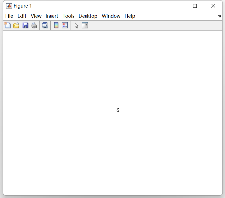
and a warning occurs:
1
2
3
4
5
6
7
8
Warning: Escaped character '\p' is not valid. See 'doc
sprintf' for supported special characters.
> In script3 (line 5)
Warning: Error updating Text.

 String scalar or character vector must have valid
 interpreter syntax:
$
which is caused by sprintf function:
1
2
3
4
5
>> sprintf("$\pi$: %.4f",3.1415)
Warning: Escaped character '\p' is not valid. See 'doc
sprintf' for supported special characters.
ans =
    "$"
But today, I found an answer to solve this problem in Blog 7, that is formatting the LaTeX syntax as well:
1
2
3
4
5
clc,clear,close all
figure("Color","w")
axes("Visible","off")
text(0.5,0.5,sprintf("%s: %.4f","$\pi$",3.1415), ...
    "Interpreter","latex")
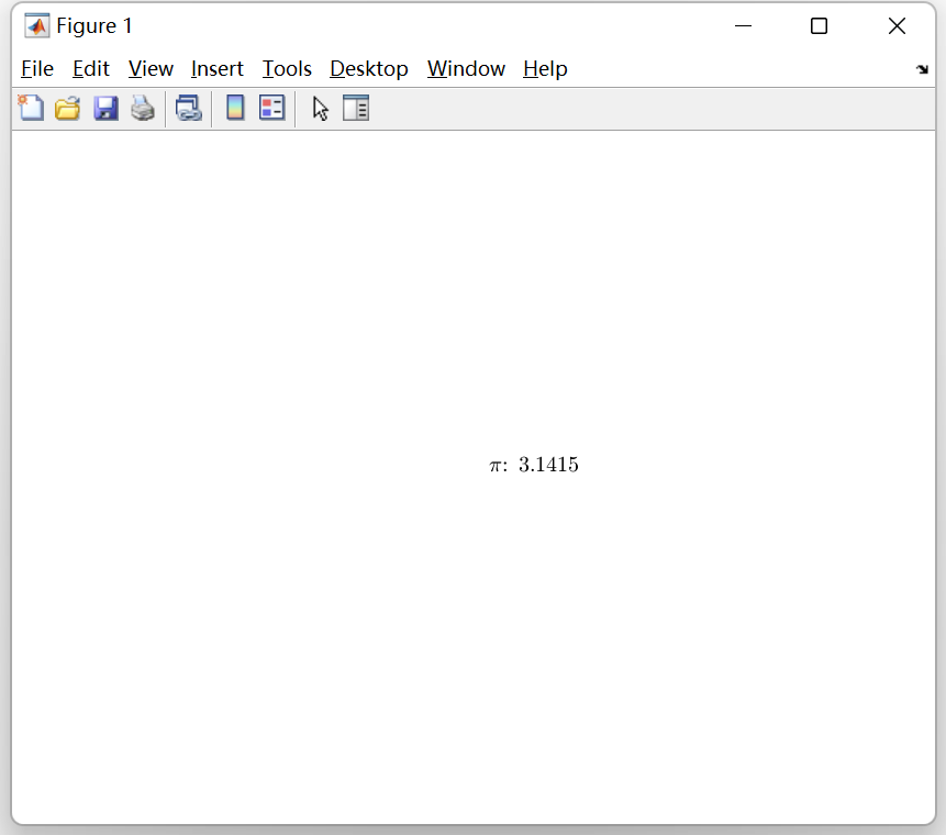
At this time, it works! Therefore, in Script 1, I adopt a similar way.
(III) LaTeX vs. TeX interpreter
For MATLAB title, text, xlabel, ylabel and other similar functions displaying text in figures, two interpreters are available for "Interpreter" property, i.e. tex and latex, and there exist two differences between these two. For example:
1
2
3
4
5
6
7
8
9
10
11
clc,clear,close all
figure("Color","w")
axes("Visible","off")
text(0.5,0.6,sprintf("%s: %.4f","$\pi$",3.1415), ...
    "Interpreter","latex","FontSize",15)
text(0.5,0.5,sprintf("%s: %.4f","\pi",3.1415), ...
    "Interpreter","latex","FontSize",15)
text(0.5,0.4,sprintf("%s: %.4f","$\pi$",3.1415), ...
    "Interpreter","tex","FontSize",15)
text(0.5,0.3,sprintf("%s: %.4f","\pi",3.1415), ...
    "Interpreter","tex","FontSize",15)
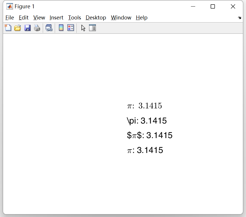
As can be seen:
(a) Identifier $ is not needed while adopting tex interpreter, but it is necessary for latex interpreter;
(b) latex interpreter will parse the whole string (see 3.1415 of first line in above figure), while tex just parse the control sequence after slash \<symbol> (see 3.1415 of third and fourth lines in above figure).
(IV) Coloring text
Coloring text in MATLAB could be realized by control sequence \color, but it should be noted that, this control sequence could ONLY be identified by tex identifier:
1
2
3
4
5
6
7
clc,clear,close all
figure("Color","w")
axes("Visible","off")
text(0.5,0.6,sprintf("%s%s: %.4f","\color{red}","$\pi$",3.1415), ...
    "Interpreter","latex","FontSize",15)
text(0.5,0.3,sprintf("%s%s: %.4f","\color{red}","\pi",3.1415), ...
    "Interpreter","tex","FontSize",15)
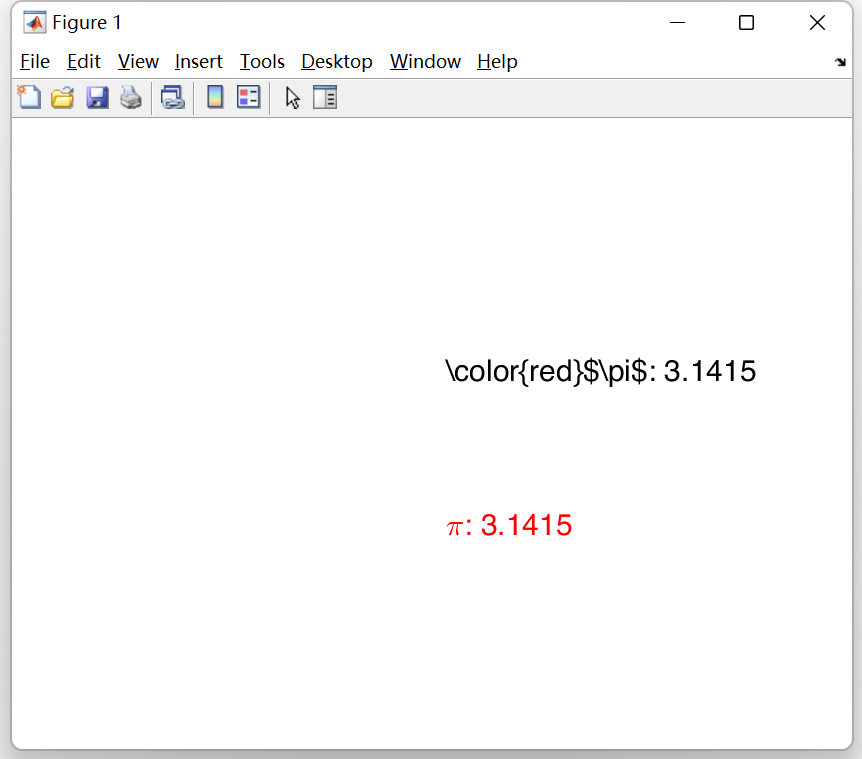
1
2
3
4
Warning: Error updating Text.

 String scalar or character vector must have valid interpreter syntax:
\color{red}$\pi$: 3.1415
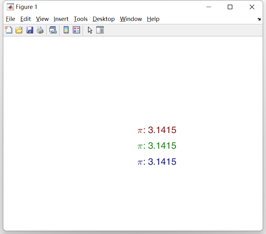
furthermore, we could specify specific RGB tuple for \color, for example 8:
1
2
3
4
5
6
7
8
9
clc,clear,close all
figure("Color","w")
axes("Visible","off")
text(0.5,0.5,sprintf("%s%s: %.4f","\color[rgb]{.5 .1 .1}","\pi",3.1415), ...
    "Interpreter","tex","FontSize",15)
text(0.5,0.4,sprintf("%s%s: %.4f","\color[rgb]{.1 .5 .1}","\pi",3.1415), ...
    "Interpreter","tex","FontSize",15)
text(0.5,0.3,sprintf("%s%s: %.4f","\color[rgb]{.1 .1 .5}","\pi",3.1415), ...
    "Interpreter","tex","FontSize",15)
At last, we look backward to Monte Carlo estimation for $\pi$. If changing the number of added points per frame (pointsPerCount of helperDrawFrame function in Script 1) from 50 to 700, a Monte Carlo simulation involving more points shows like:
It can be seen that, using this simulation way to calculate $\pi$ converge very very slowly.
References
-
MATLAB Flipbook Mini Hack Contest Description, Rules, and Terms - MATLAB. ˄
-
Create Animation in MATLAB: Render
.gifand.aviFile - What a starry night~. ˄ -
Monte-Carlo estimation of pi - MATLAB Flipbook Mini Hack. ˄ ˄2 ˄3
-
MATLAB persistent: Define persistent variable - MathWorks. ˄ ˄2
-
MATLAB
sprintfFunction andtitleFunction - What a starry night~. ˄ -
Predefining colors for in-text coloring - MATLAB Answers - MATLAB Central. ˄