LaTeX TikZ shape Option and shapes Library
The shape option
When making diagrams using LaTeX TikZ, there is a shape option1 (2, p. 225, p. 228):
/tikz/shape=⟨shape name⟩ (no default, initially rectangle)
Select the shape either of the current node or, when this option is not given inside a node but somewhere outside, the shape of all nodes in the current scope.
Since this option is used often, you can leave out the shape=. When TikZ encounters an option like circle that it does not know, it will, after everything else has failed, check whether this option is the name of some shape. If so, that shape is selected as if you had said shape=⟨shape name⟩.
By default, the following shapes are available: rectangle, circle, coordinate.
For example:
1
2
3
4
5
6
7
8
9
10
11
12
13
14
15
16
\documentclass[border=10pt]{standalone}
\usepackage{tikz}

\begin{document}

\begin{tikzpicture}
\draw (0,0)node[draw]{A} -- (1,1)node[draw]{B};

\path node at (4,2)[shape=circle,draw]{}
      node at (4,1)[shape=circle,draw]{}
      node at (4,0)[shape=circle,draw]{}
      node at (5,1)[shape=rectangle,draw]{}
      node at (3,1)[shape=rectangle,draw]{};
\end{tikzpicture}

\end{document}

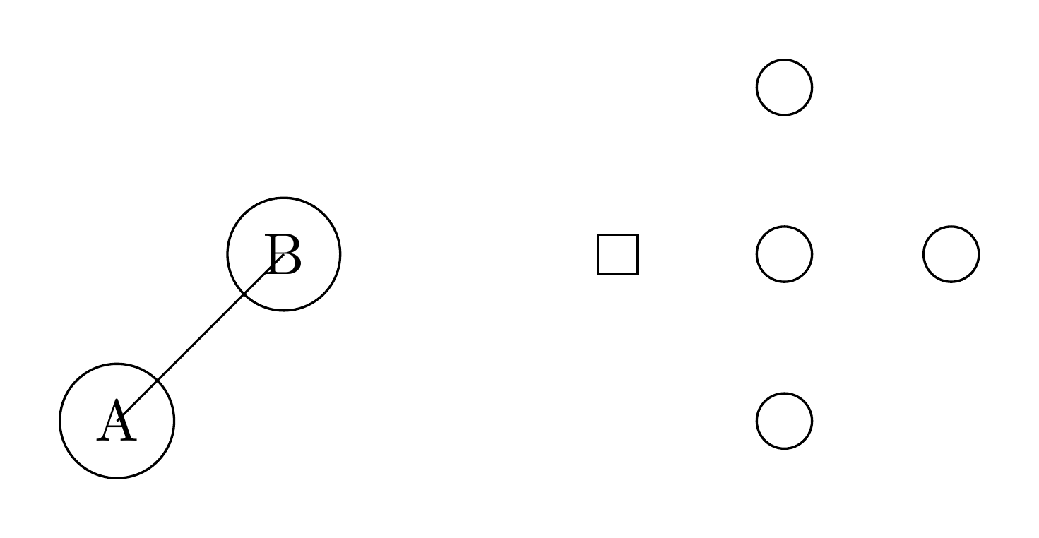
Note that, the draw option is necessary, and it means that, the circle, or other shapes, is to be drawn, but not filled or otherwise used (2, p. 52). If we don’t use it, the resulting figure will become:
1
2
3
4
5
6
7
8
9
10
11
12
13
14
15
16
\documentclass[border=10pt]{standalone}
\usepackage{tikz}

\begin{document}

\begin{tikzpicture}
\draw (0,0)node{A} -- (1,1)node{B};

\path node at (4,2)[shape=circle]{}
      node at (4,1)[shape=circle]{}
      node at (4,0)[shape=circle]{}
      node at (5,1)[shape=rectangle]{}
      node at (3,1)[shape=rectangle]{};
\end{tikzpicture}

\end{document}
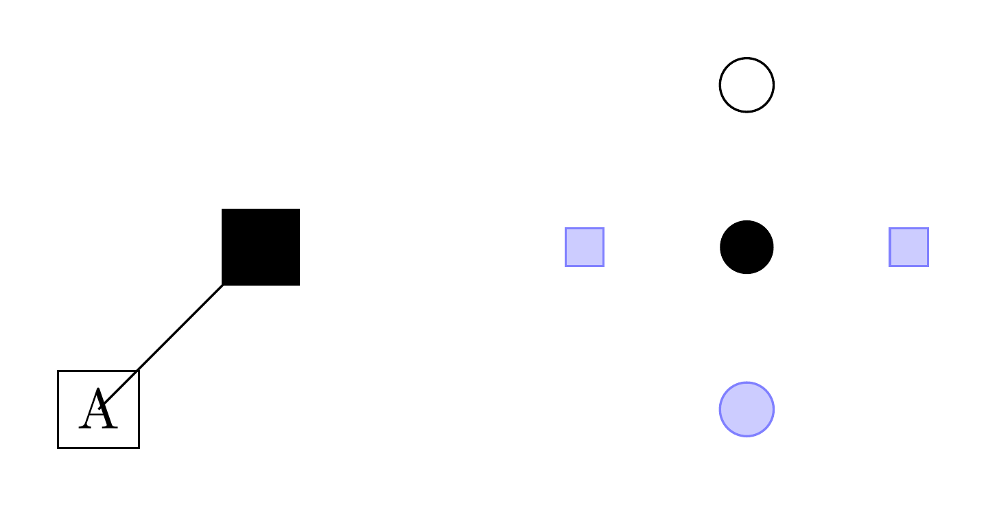
By the way, we can fill the circle, or other shapes, and furthermore set the border color by the draw option:
1
2
3
4
5
6
7
8
9
10
11
12
13
14
15
16
\documentclass[border=10pt]{standalone}
\usepackage{tikz}

\begin{document}

\begin{tikzpicture}
\draw (0,0)node[draw]{A} -- (1,1)node[fill]{B};

\path node at (4,2)[shape=circle,draw]{}
      node at (4,1)[shape=circle,fill]{}
      node at (4,0)[shape=circle,draw=blue!50,fill=blue!20]{}
      node at (5,1)[shape=rectangle,draw=blue!50,fill=blue!20]{}
      node at (3,1)[shape=rectangle,draw=blue!50,fill=blue!20]{};
\end{tikzpicture}

\end{document}
According to the description from the documentation showed above, we can directly set the shape option after the tikzpicture environment to set the shape of each node in the whole environment:
1
2
3
4
5
6
7
8
9
10
11
12
13
14
15
16
\documentclass[border=10pt]{standalone}
\usepackage{tikz}

\begin{document}

\begin{tikzpicture}[shape=circle]
\draw (0,0)node[draw]{A} -- (1,1)node[draw]{B};

\path node at (4,2)[draw]{}
      node at (4,1)[draw]{}
      node at (4,0)[draw]{}
      node at (5,1)[draw]{}
      node at (3,1)[shape=rectangle,draw]{};
\end{tikzpicture}

\end{document}
or after the \draw and \path etc. commands to set locally:
1
2
3
4
5
6
7
8
9
10
11
12
13
14
15
16
\documentclass[border=10pt]{standalone}
\usepackage{tikz}

\begin{document}

\begin{tikzpicture}
\draw[shape=circle] (0,0)node[draw]{A} -- (1,1)node[draw]{B};

\path[shape=circle] node at (4,2)[draw]{}
      node at (4,1)[draw]{}
      node at (4,0)[draw]{}
      node at (5,1)[draw]{}
      node at (3,1)[draw]{};
\end{tikzpicture}

\end{document}
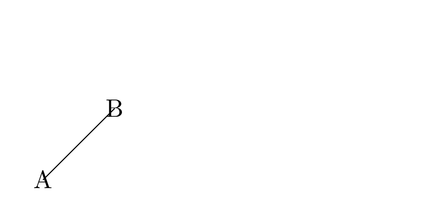
At last, again, as described in the documentation cited above, we can leave out shape=, i.e., abbreviate shape=circle as circle etc.:
1
2
3
4
5
6
7
8
9
10
11
12
13
14
15
16
\documentclass[border=10pt]{standalone}
\usepackage{tikz}

\begin{document}

\begin{tikzpicture}
\draw (0,0)node[draw]{A} -- (1,1)node[draw]{B};

\path node at (4,2)[circle,draw]{}
      node at (4,1)[circle,draw]{}
      node at (4,0)[circle,draw]{}
      node at (5,1)[rectangle,draw]{}
      node at (3,1)[rectangle,draw]{};
\end{tikzpicture}

\end{document}
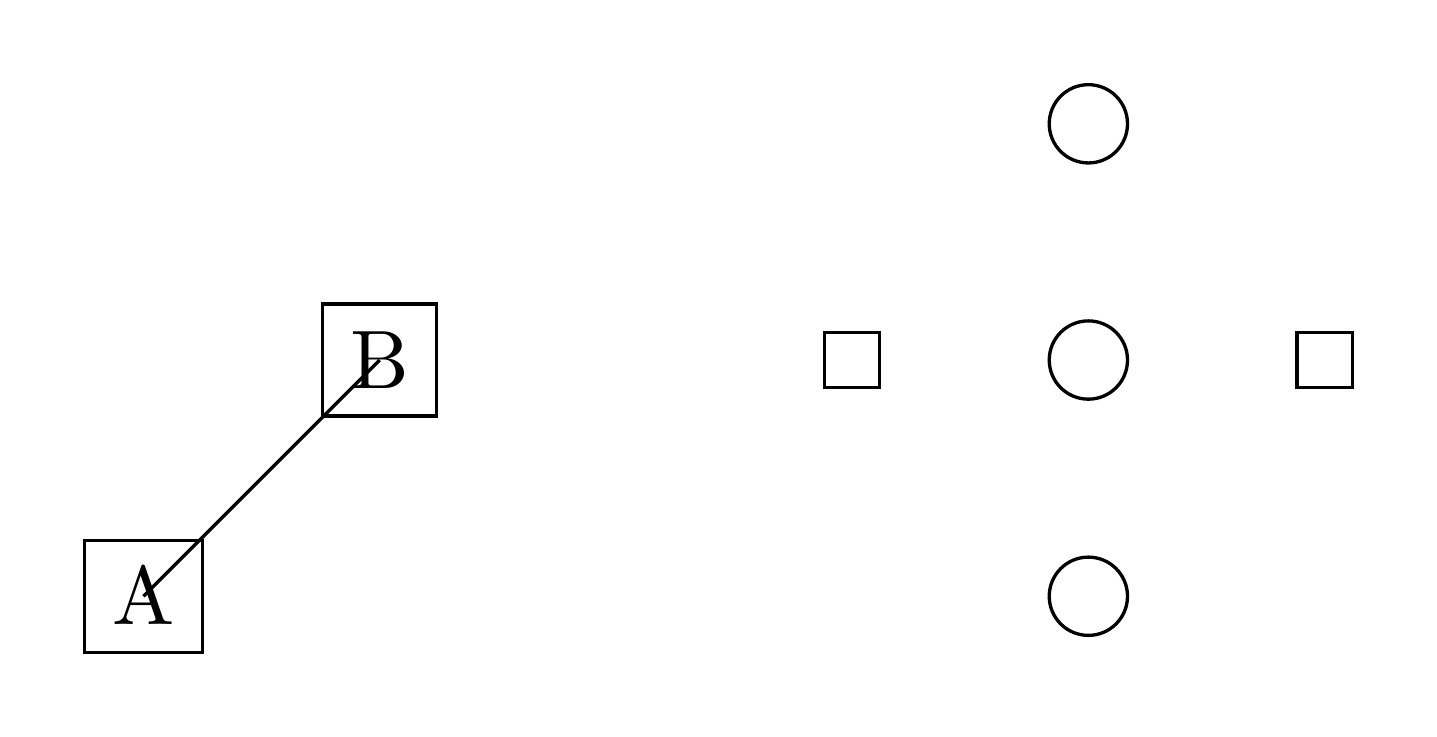
which is the same as Fig. 1.
The TikZ shapes library
By default, there are only three standard shapes, rectangle, circle, and coordinate. Luckily, the TikZ shape library, including several sublibraries, provides more shapes (2, p. 785):
In addition to the standard shapes rectangle, circle and coordinate, there exist a number of additional shapes defined in different shape libraries. Most of these shapes have been contributed by Mark Wibrow. In the present section, these shapes are described. Note that the library shapes is provided for compatibility only. Please include sublibraries like shapes.geometric or shapes.misc directly.
The shapes.geometric sublibrary
The shapes.geometric sublibrary provides shapes such as diamond, ellipse, trapezium, semicircle, regular polygon, star, isosceles triangle, kite, dart, circular sector, cylinder (2, pp. 786-801):
1
2
3
4
5
6
7
8
9
10
11
12
13
14
15
16
17
18
19
20
21
\documentclass[border=10pt]{standalone}
\usepackage{tikz}
\usetikzlibrary{shapes.geometric}

\begin{document}

\begin{tikzpicture}
\path node at (0,0)[diamond,draw]{}
	  node at (1,0)[ellipse,draw]{}
	  node at (2,0)[trapezium,draw]{}
	  node at (3,0)[semicircle,draw]{}
	  node at (4,0)[regular polygon,draw]{}
	  node at (5,0)[star,draw]{}
	  node at (0,-1)[isosceles triangle,draw]{}
	  node at (1,-1)[kite,draw]{}
	  node at (2,-1)[dart,draw]{}
	  node at (3,-1)[circular sector,draw]{}
	  node at (4,-1)[cylinder,draw]{};
\end{tikzpicture}

\end{document}

and each shape has its own keys and anchors.
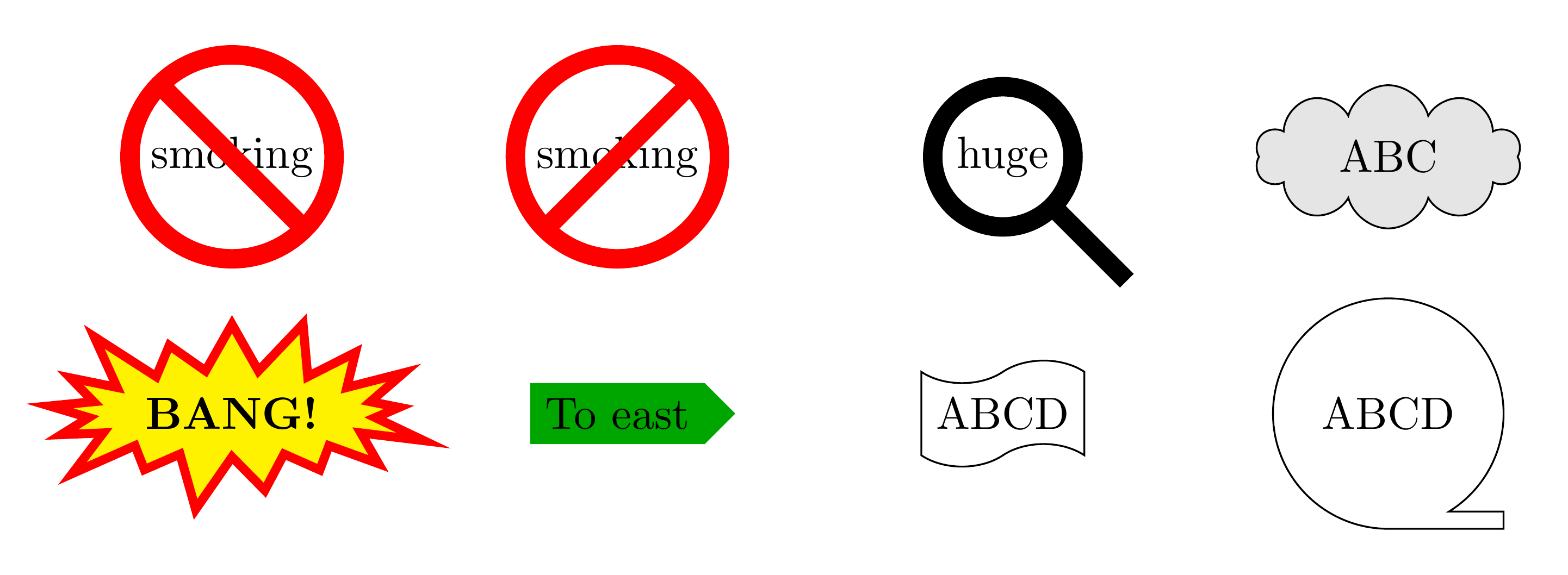
The shapes.symbols sublibrary
1
2
3
4
5
6
7
8
9
10
11
12
13
14
15
16
17
18
\documentclass[border=10pt]{standalone}
\usepackage{tikz}
\usetikzlibrary{shapes.symbols}

\begin{document}

\begin{tikzpicture}
\path node at (0,0)[correct forbidden sign,line width=1ex,draw=red,fill=white]{smoking}
	  node at (3,0)[forbidden sign,line width=1ex,draw=red,fill=white]{smoking}
	  node at (6,0)[magnifying glass,line width=1ex,draw]{huge}
	  node at (9,0)[cloud,draw,fill=gray!20,aspect=3]{ABC}
	  node at (0,-2)[starburst,draw,fill=yellow,draw=red,line width=2pt]{\bf BANG!}
	  node at (3,-2)[signal,fill=green!65!black,signal to=east]{To east}
	  node at (6,-2)[tape,draw]{ABCD}
	  node at (9,-2)[magnetic tape,draw]{ABCD};
\end{tikzpicture}

\end{document}
The shapes.arrows sublibrary
1
2
3
4
5
6
7
8
9
10
11
12
13
\documentclass[border=10pt]{standalone}
\usepackage{tikz}
\usetikzlibrary{shapes.arrows}

\begin{document}

\begin{tikzpicture}
\path node at (0,0)[single arrow,draw]{right}
      node at (3,0)[double arrow,draw]{Left or Right}
      node at (6,0)[arrow box,draw]{A};
\end{tikzpicture}

\end{document}

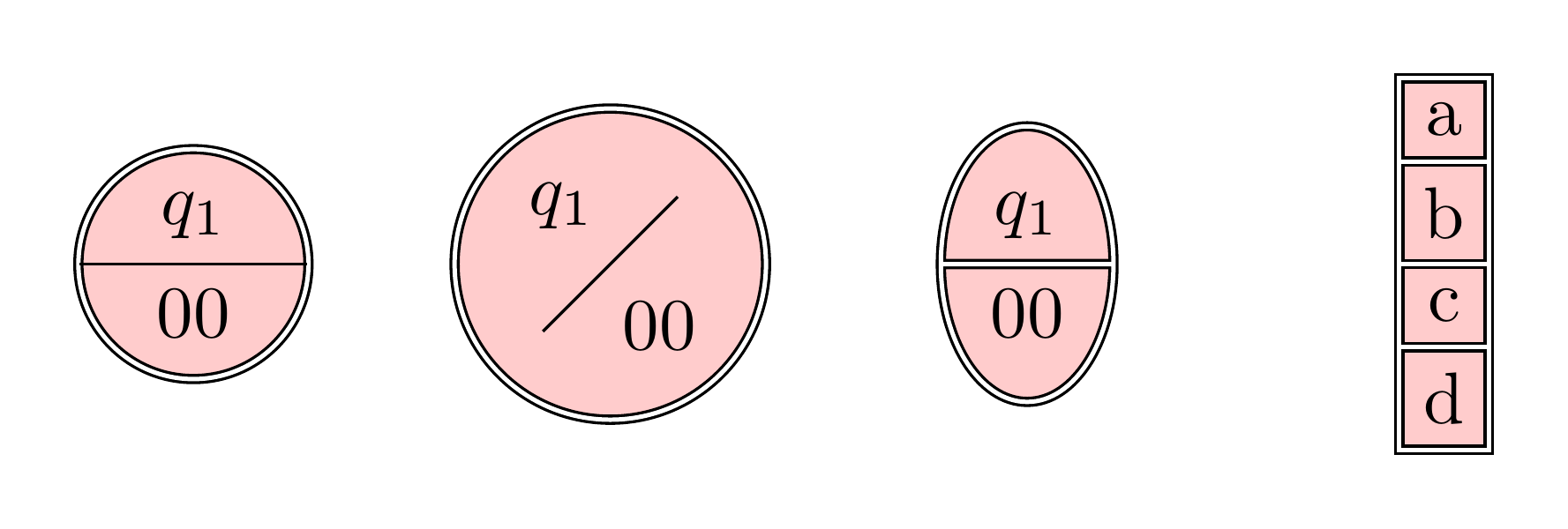
The shapes.multipart sublibrary
1
2
3
4
5
6
7
8
9
10
11
12
13
14
15
\documentclass[border=10pt]{standalone}
\usepackage{tikz}
\usetikzlibrary{shapes.multipart}

\begin{document}

\begin{tikzpicture}
\path node at (0,0)[circle split,draw,double,fill=red!20]{$q_1$\nodepart{lower}$00$}
      node at (2,0)[circle solidus,draw,double,fill=red!20]{$q_1$\nodepart{lower}$00$}
      node at (4,0)[ellipse split,draw,double,fill=red!20]{$q_1$\nodepart{lower}$00$}
      node at (6,0)[rectangle split,draw,double,fill=red!20]{a\nodepart{two}b\nodepart{three}c\nodepart{four}d\nodepart{five}e}
      ;
\end{tikzpicture}

\end{document}
The shapes.callouts sublibrary
1
2
3
4
5
6
7
8
9
10
11
12
13
\documentclass[border=10pt]{standalone}
\usepackage{tikz}
\usetikzlibrary{shapes.callouts}

\begin{document}

\begin{tikzpicture}
\path node at (0,0)[rectangle callout,draw]{Hello!}
      node at (2,0)[ellipse callout,draw]{Hello!}
      node at (4,0)[cloud callout,draw]{Hello!};
\end{tikzpicture}

\end{document}

The shapes.misc sublibrary
1
2
3
4
5
6
7
8
9
10
11
12
13
14
\documentclass[border=10pt]{standalone}
\usepackage{tikz}
\usetikzlibrary{shapes.misc}

\begin{document}

\begin{tikzpicture}
\path node at (0,0)[cross out,draw=red]{cross out}
      node at (2,0)[strike out,draw=red]{strike out}
      node at (4,0)[rounded rectangle,draw=red]{Hello}
      node at (6,0)[chamfered rectangle,white,fill=red,double=red,draw,very thick]{STOP!};
\end{tikzpicture}

\end{document}

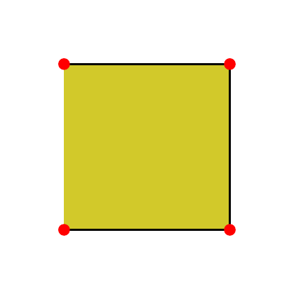
Specify shape=coordinate
Kind of different other shapes, shape=coordinate will create an invisible zero-dimensional point with no size at the specified position, which is like the “point”3 in the mathematical meaning. Here is an example (2, 228):
1
2
3
4
5
6
7
8
9
10
11
12
13
14
15
16
17
18
19
20
21
22
23
24
25
26
27
28
\documentclass[border=10pt]{standalone}
\usepackage{tikz}

\begin{document}

\begin{tikzpicture}[every node/.style={draw}]
\path[shape=rectangle]
	(0,0) node(a1){} (1,0) node(a2){}
	(1,1) node(a3){} (0,1) node(a4){};
\filldraw[fill=yellow!80!black] (a1) -- (a2) -- (a3) -- (a4);

\path[yshift=-1.5cm,shape=coordinate]
	(0,0) node(a1){} (1,0) node(a2){}
	(1,1) node(a3){} (0,1) node(a4){};
\filldraw[fill=yellow!80!black] (a1) -- (a2) -- (a3) -- (a4);

\path[xshift=1.5cm,shape=circle]
	(0,0) node(a1){} (1,0) node(a2){}
	(1,1) node(a3){} (0,1) node(a4){};
\filldraw[fill=yellow!80!black] (a1) -- (a2) -- (a3) -- (a4);

\path[xshift=1.5cm,yshift=-1.5cm,shape=coordinate]
	(0,0) node(a1){} (1,0) node(a2){}
	(1,1) node(a3){} (0,1) node(a4){};
\filldraw[fill=yellow!80!black] (a1) -- (a2) -- (a3) -- (a4);
\end{tikzpicture}

\end{document}
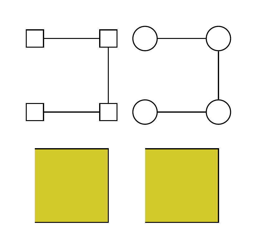
We can see that, here specifying shape=coordinate is “… useful since, normally, the line shortening causes paths to be segmented and they cannot be used for filling” (2, p. 228).
Besides, we can use equivalent syntax (<position>) coordinate(<name>) instead in the \path command:
1
2
3
4
5
6
7
8
9
10
11
12
13
14
15
16
17
18
19
20
21
22
23
24
25
26
27
28
\documentclass[border=10pt]{standalone}
\usepackage{tikz}

\begin{document}

\begin{tikzpicture}[every node/.style={draw}]
\path[shape=rectangle]
	(0,0) node(a1){} (1,0) node(a2){}
	(1,1) node(a3){} (0,1) node(a4){};
\filldraw[fill=yellow!80!black] (a1) -- (a2) -- (a3) -- (a4);

\path[yshift=-1.5cm]
	(0,0) coordinate(a1) (1,0) coordinate(a2)
	(1,1) coordinate(a3) (0,1) coordinate(a4);
\filldraw[fill=yellow!80!black] (a1) -- (a2) -- (a3) -- (a4);

\path[xshift=1.5cm,shape=circle]
	(0,0) node(a1){} (1,0) node(a2){}
	(1,1) node(a3){} (0,1) node(a4){};
\filldraw[fill=yellow!80!black] (a1) -- (a2) -- (a3) -- (a4);

\path[xshift=1.5cm,yshift=-1.5cm]
	(0,0) coordinate(a1) (1,0) coordinate(a2)
	(1,1) coordinate(a3) (0,1) coordinate(a4);
\filldraw[fill=yellow!80!black] (a1) -- (a2) -- (a3) -- (a4);
\end{tikzpicture}

\end{document}
or use the \coordinate command:
1
2
3
4
5
6
7
8
9
10
11
12
13
14
15
16
17
18
19
20
21
22
23
24
25
26
27
28
29
30
\documentclass[border=10pt]{standalone}
\usepackage{tikz}

\begin{document}

\begin{tikzpicture}[every node/.style={draw}]
\path[shape=rectangle]
	(0,0) node(a1){} (1,0) node(a2){}
	(1,1) node(a3){} (0,1) node(a4){};
\filldraw[fill=yellow!80!black] (a1) -- (a2) -- (a3) -- (a4);

\coordinate[yshift=-1.5cm] (a1) at (0,0);
\coordinate[yshift=-1.5cm] (a2) at (1,0);
\coordinate[yshift=-1.5cm] (a3) at (1,1);
\coordinate[yshift=-1.5cm] (a4) at (0,1);
\filldraw[fill=yellow!80!black] (a1) -- (a2) -- (a3) -- (a4);

\path[xshift=1.5cm,shape=circle]
	(0,0) node(a1){} (1,0) node(a2){}
	(1,1) node(a3){} (0,1) node(a4){};
\filldraw[fill=yellow!80!black] (a1) -- (a2) -- (a3) -- (a4);

\coordinate[xshift=1.5cm,yshift=-1.5cm] (a1) at (0,0);
\coordinate[xshift=1.5cm,yshift=-1.5cm] (a2) at (1,0);
\coordinate[xshift=1.5cm,yshift=-1.5cm] (a3) at (1,1);
\coordinate[xshift=1.5cm,yshift=-1.5cm] (a4) at (0,1);
\filldraw[fill=yellow!80!black] (a1) -- (a2) -- (a3) -- (a4);
\end{tikzpicture}

\end{document}
Both scripts will render the same figure as Fig. 2.
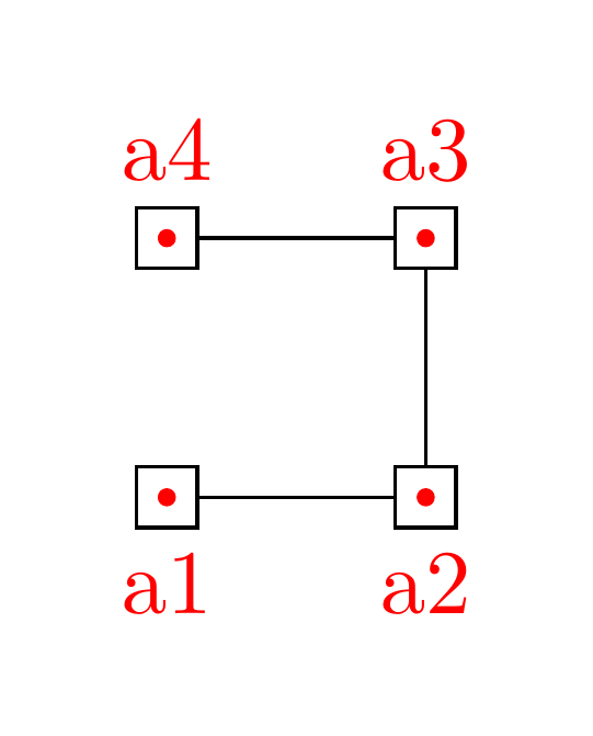
In addition, we should note that, when we specify [shape=coordinate] for the whole tikzpicture environment, something may become not as we expected, because each node in this environment, by default, will be viewed as a coordinate, which is a zero-dimensional point. For example, in the following example, the text we annotate for the filled circles are invisible:
1
2
3
4
5
6
7
8
9
10
11
12
13
14
15
16
17
18
19
20
21
22
23
24
25
26
27
28
\documentclass[border=10pt,tikz]{standalone}
\usepackage{tikz}

\begin{document}

\begin{tikzpicture}
\path (0,0) node(a1)[draw]{} (1,0) node(a2)[draw]{}
      (1,1) node(a3)[draw]{} (0,1) node(a4)[draw]{};
\filldraw[fill=yellow!80!black] (a1) -- (a2) -- (a3) -- (a4);

\fill[red] (a1) circle (1pt) node[below=0.1cm]{a1};
\fill[red] (a2) circle (1pt) node[below=0.1cm]{a2};
\fill[red] (a3) circle (1pt) node[above=0.1cm]{a3};
\fill[red] (a4) circle (1pt) node[above=0.1cm]{a4};
\end{tikzpicture}

\begin{tikzpicture}[shape=coordinate] % NOTE here is the only difference.
\path (0,0) node(a1)[draw]{} (1,0) node(a2)[draw]{}
      (1,1) node(a3)[draw]{} (0,1) node(a4)[draw]{};
\filldraw[fill=yellow!80!black] (a1) -- (a2) -- (a3) -- (a4);

\fill[red] (a1) circle (1pt) node[below=0.1cm]{a1};
\fill[red] (a2) circle (1pt) node[below=0.1cm]{a2};
\fill[red] (a3) circle (1pt) node[above=0.1cm]{a3};
\fill[red] (a4) circle (1pt) node[above=0.1cm]{a4};
\end{tikzpicture}

\end{document}
References