LaTeX CircuiTikz Examples (II)

Jun. 01, 2025 • Updated Jun. 06, 2025

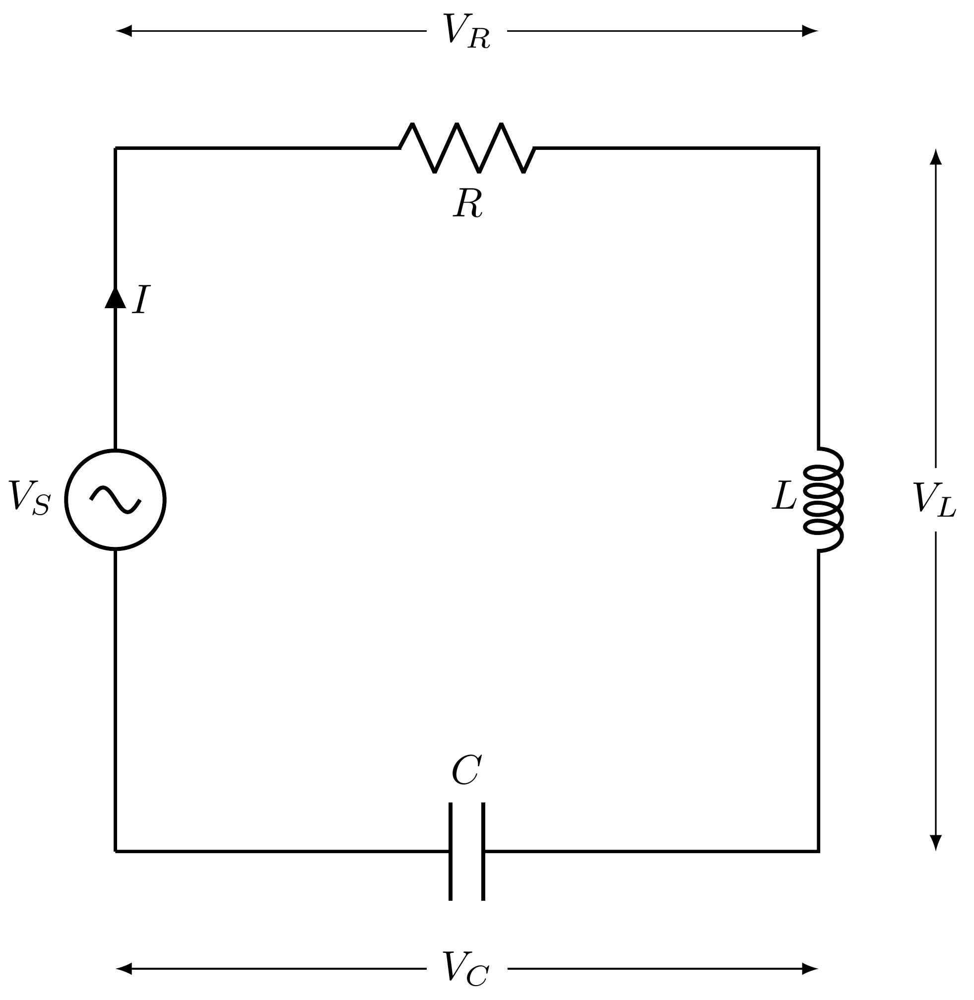
Example 1: RLC Circuit

Example 1: RLC Circuit¹

\documentclass{standalone}
\usepackage{circuitikz}
\ctikzset{bipoles/thickness=1.2}

\newcommand{\midlabelline}[3]{
   \node (midlabel) at ($ (#1)!.5!(#2) $) {#3};
   \draw[latex-] (#1) --  (midlabel);
   \draw[-latex] (midlabel) -- (#2);
}

\begin{document}
\begin{circuitikz}
	% Circuit
	\draw[line width=0.8]
	  (2,7) to [sinusoidal voltage source, l_=$V_S$, i=$I$] (2,1)
	  (2,7) to [resistor, l_=$R$] ++(6,0) to [inductor, l_=$L$] ++(0,-6) to [capacitor, l_=$C$] +(-6,0);
 
	% Voltage Infos
	\midlabelline{2,8}{8,8}{$V_R$}
	\midlabelline{9,7}{9,1}{$V_L$}
	\midlabelline{2,0}{8,0}{$V_C$}
\end{circuitikz}
\end{document}

Here is an annotated version:

\documentclass{standalone}
\usepackage{circuitikz}
\ctikzset{bipoles/thickness=1.2}

\newcommand{\midlabelline}[3]{
   \node (midlabel) at ($ (#1)!.5!(#2) $) {#3};
   \draw[latex-] (#1) --  (midlabel);
   \draw[-latex] (midlabel) -- (#2);
}

\begin{document}
\begin{circuitikz}
	\draw [help lines,step=1cm] (0,0) grid (10,8); % Helper lines on the background
	
	% Circuit
	\draw[line width=0.8]
	  (2,7) to [sinusoidal voltage source, l_=$V_S$, i=$I$] (2,1)
	  (2,7) to [resistor, l_=$R$] ++(6,0) to [inductor, l_=$L$] ++(0,-6) to [capacitor, l_=$C$] +(-6,0);
 
	% Voltage Infos
	\midlabelline{2,8}{8,8}{$V_R$}
	\midlabelline{9,7}{9,1}{$V_L$}
	\midlabelline{2,0}{8,0}{$V_C$}
	
	\fill [red] (2,7) circle (1pt) node[left=0.1cm]{(2,7)};
	\fill [red] (2,1) circle (1pt) node[left=0.1cm]{(2,1)};
	\fill [red] (8,7) circle (1pt) node[right=0.1cm]{(8,7)};
	\fill [red] (8,1) circle (1pt) node[right=0.1cm]{(8,1)};
	
	\fill [red] (2,8) circle (1pt) node[left=0.1cm]{(2,8)};
	\fill [red] (8,8) circle (1pt) node[right=0.1cm]{(8,8)};
	\fill [red] (9,1) circle (1pt) node[right=0.1cm, below=0.1cm]{(9,1)};
	\fill [red] (9,7) circle (1pt) node[right=0.1cm]{(9,7)};
	\fill [red] (2,0) circle (1pt) node[left=0.1cm]{(2,0)};
	\fill [red] (8,0) circle (1pt) node[right=0.1cm]{(8,0)};
\end{circuitikz}
\end{document}

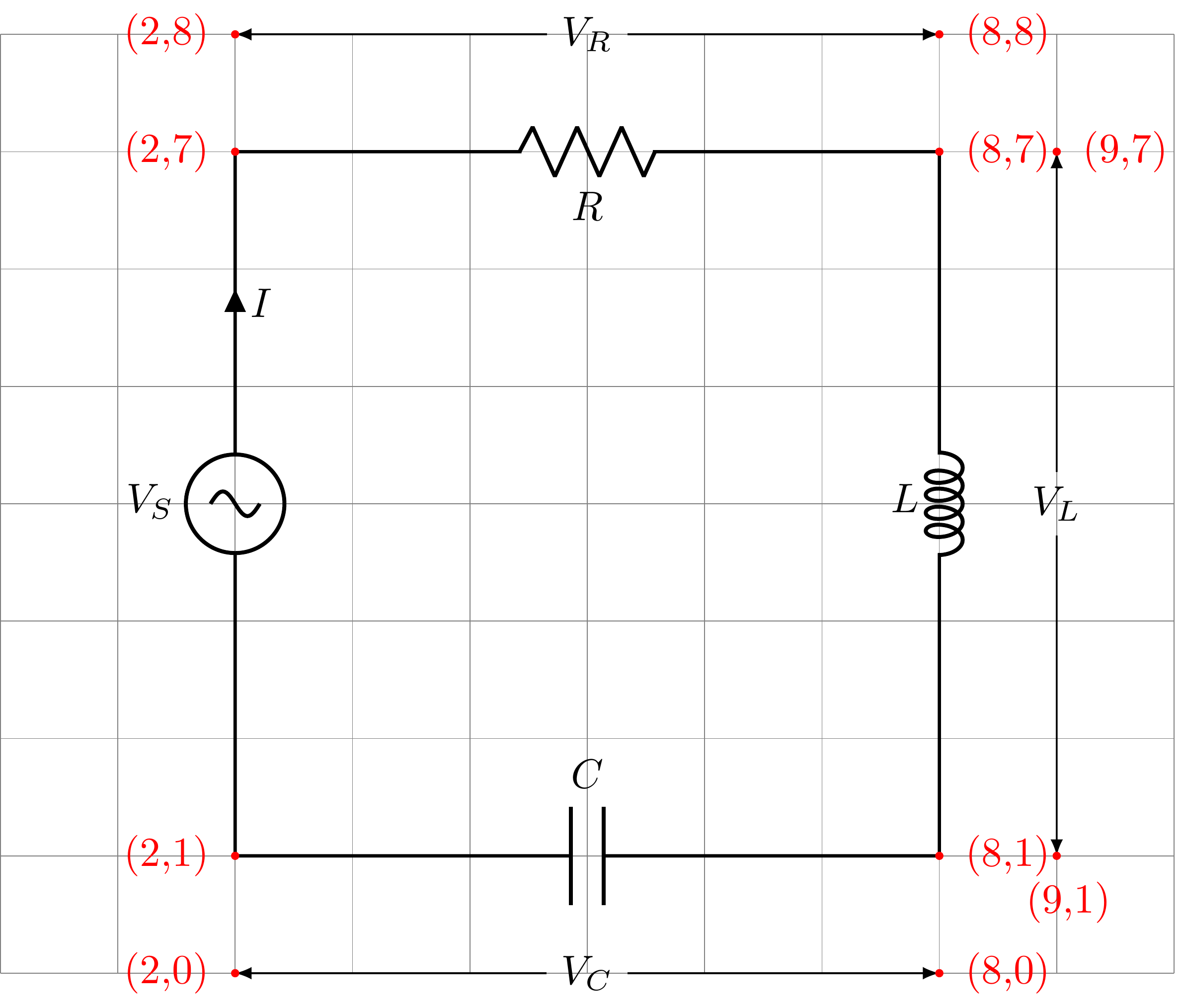
In this example, the way of defining a new command facilitates labeling text next to the component:

\newcommand{\midlabelline}[3]{
   \node (midlabel) at ($ (#1)!.5!(#2) $) {#3};
   \draw[latex-] (#1) --  (midlabel);
   \draw[-latex] (midlabel) -- (#2);
}

Example 2: Buck, Buck-Boost, and Boost Converter

Example 2-1: Buck Converter

Example 2-1: Buck Converter²

% Buck Converter
% This DC-DC converter decreases the voltage level from input to output

% Designed by: Amir Ostadrahimi

\documentclass[border=5pt]{standalone}
\usepackage{tikz}
\usepackage[american,cuteinductors,smartlabels]{circuitikz} % A package to draw electrical networks with TikZ

%-- the dimensions of the elements can be changed here
\ctikzset{bipoles/thickness=0.7}
\ctikzset{bipoles/length=1.5cm}
\ctikzset{bipoles/resistor/width=0.7}
\ctikzset{bipoles/resistor/height=0.25}
\ctikzset{bipoles/diode/height=0.3}
\ctikzset{bipoles/diode/width=0.3}
\ctikzset{tripoles/thickness=0.7}
\ctikzset{bipoles/battery1/height=0.7}

%settings for fonts and lines
\tikzstyle{every node}=[font=\Large]
\tikzstyle{every path}=[line width=0.9 pt, line cap=round, line join=round]

\begin{document}

\begin{circuitikz}
%------ Converter
\coordinate  (VBottom) at (0,0); %%VBottom stands for voltage source bottom and is located on (0,0)

\draw (VBottom) to [battery1, l=$V_{in}$, invert] ++(0,3) coordinate (VTop); % "battery1" is to insert voltage source, instead of it, you can use "battery", "battery2", or "V".
% the " l=$V_{in}$" is for label. You can use  "l_=$V_{in}$" or "l^=$V_{in}$" to change its location. 
%"invert" changes the polarity of the source. (VTop) stands for voltage top.
% to change size of the voltage source, we can modify "\ctikzset{bipoles/battery1/height=0.7}", at the beginning of the documents

\draw (VTop) to [short] ++(0.8,0) node [nigbt, anchor=C, rotate=90, label={[yshift=-1.5 cm] \normalsize $IGBT$}] (nigbt1){}; % here we used an N-channel IGBT using "nigbt". Alternatively, we could use "pigbt", "nmos", "pmos" and so on.


\draw (nigbt1.E) to [short]++(0.5,0) coordinate (DiodeTop) to [short]++(0.5,0) to [L, l_=$L$, v^=$v_L$, i>_=$i_L$]++ (2,0) coordinate (InductorRight);  % "i>_=$i_L$ " is for showing the current of the element, by using "^" we can change its location and bring it at the input and the output of the element. By using  "<"  and  ">"  we can change its direction. And finally by using "_" we can change its vertical location. Using "coordinate (DiodeTop) " we considered a connection point to the diode.

\draw   (DiodeTop) to [D*, invert] (DiodeTop|-VBottom); %Using  " (DiodeTop|-VBottom)" the diode will be continued till the intersection of the vertical line from (DiodeTop) and the horizontal line from (VBottom). Here, "invert" is used to change the direction of the diode and "*" is used to change type of the diode to filled-black diode

\draw (InductorRight) to [short]++(0.5,0)  coordinate (CapacitorTop) to [C, l_=$C$, i>^=$i_c$](CapacitorTop|-VBottom);  %Using  " (CapacitorTop|-VBottom)" the diode will be continued till the intersection of the vertical line from (CapacitorTop) and the horizontal line from (VBottom)

\draw  (CapacitorTop) to [short]++(1.5,0)  coordinate (ResistorTop) to [R, l_=$R$, v^=$V_{out}$](ResistorTop|-VBottom) coordinate (ResistorBottom)

(ResistorBottom)-- (VBottom);


%------ Conversion Ratio

\coordinate [label={ [xshift=0, yshift=0] \large $ M(D)=\frac{V_{out}}{V_{in}}=D;$ \large $0 \leq D \leq 1$ }] (M) at (3,-1);

%%------ Curve

\def\xo{2} % Axes of origin
\def\yo{-7} % Axes of origin
\def\length {5} % length of the axes
\def\N{200} %number of samples

\coordinate [label={ [xshift=-5, yshift=-12] \normalsize$0$ }] (origin) at (\xo,\yo); %

\draw[->] (\xo -0.2, \yo) -- ++(\length,0) node[right] {\small $D$};
\draw[->] (\xo,\yo -0.2) -- ++(0, \length) node[above] {\small $M(D)$};
\draw plot[samples=\N, domain=0:4, xshift=\xo cm, yshift=\yo cm] (\x, \x);

\draw (\xo, \yo) ++(2.5,0) node [below] (halfx){\normalsize $0.5$};
\draw (\xo, \yo) ++(0,2.5) node [left] (halfy){\normalsize $0.5$};
\draw [dashed] (halfx)|-(halfy);
\end{circuitikz}

\end{document}

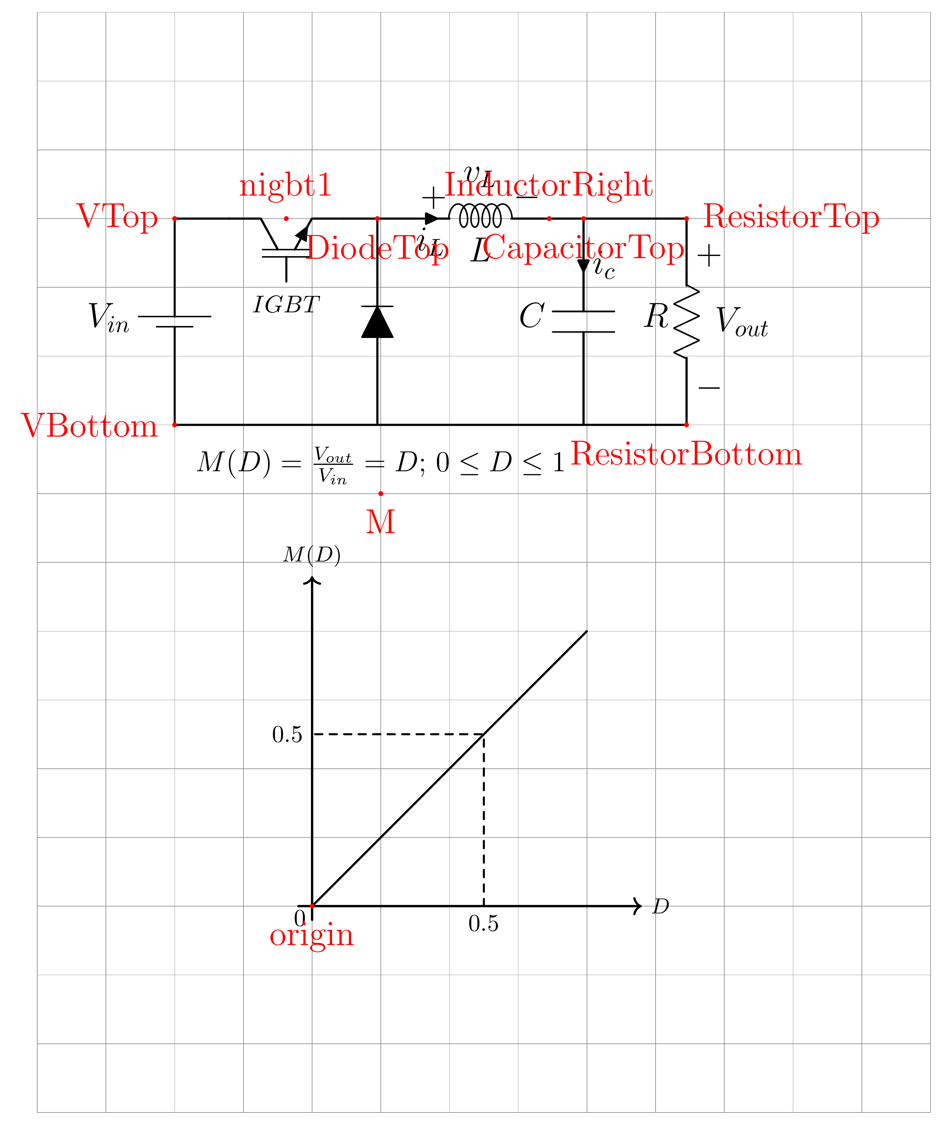
Here is an annotated version:

% Buck Converter
% This DC-DC converter decreases the voltage level from input to output
% Designed by: Amir Ostadrahimi
\documentclass[border=5pt]{standalone}
\usepackage{tikz}
\usepackage[american,cuteinductors,smartlabels]{circuitikz} % A package to draw electrical networks with TikZ

% the dimensions of the elements can be changed here
\ctikzset{bipoles/thickness=0.7}
\ctikzset{bipoles/length=1.5cm}
\ctikzset{bipoles/resistor/width=0.7}
\ctikzset{bipoles/resistor/height=0.25}
\ctikzset{bipoles/diode/height=0.3}
\ctikzset{bipoles/diode/width=0.3}
\ctikzset{tripoles/thickness=0.7}
\ctikzset{bipoles/battery1/height=0.7}

%settings for fonts and lines
\tikzstyle{every node}=[font=\Large]
\tikzstyle{every path}=[line width=0.9 pt, line cap=round, line join=round]

\begin{document}

\begin{circuitikz}
\draw [help lines,step=1cm] (-2,-10) grid (11,6); % Helper lines on the background

% Converter
\coordinate  (VBottom) at (0,0);
% VBottom stands for voltage source bottom and is located on (0,0)

\draw (VBottom) to [battery1, l=$V_{in}$, invert] ++(0,3) coordinate (VTop);
% "battery1" is to insert voltage source, instead of it, you can use "battery", "battery2", or "V".
% the " l=$V_{in}$" is for label. You can use  "l_=$V_{in}$" or "l^=$V_{in}$" to change its location. 
%"invert" changes the polarity of the source. (VTop) stands for voltage top.
% to change size of the voltage source, we can modify "\ctikzset{bipoles/battery1/height=0.7}", at the beginning of the documents

\draw (VTop) to [short] ++(0.8,0) node [nigbt, anchor=C, rotate=90, label={[yshift=-1.5 cm] \normalsize $IGBT$}] (nigbt1){};
% here we used an N-channel IGBT using "nigbt". Alternatively, we could use "pigbt", "nmos", "pmos" and so on.

\draw (nigbt1.E) to [short]++(0.5,0) coordinate (DiodeTop) to [short] ++(0.5,0) to [L, l_=$L$, v^=$v_L$, i>_=$i_L$] ++(2,0) coordinate (InductorRight);
% "i>_=$i_L$ " is for showing the current of the element, by using "^" we can change its location and bring it at the input and the output of the element. By using  "<"  and  ">"  we can change its direction. And finally by using "_" we can change its vertical location. Using "coordinate (DiodeTop) " we considered a connection point to the diode.

\draw   (DiodeTop) to [D*, invert] (DiodeTop|-VBottom);
% Using  " (DiodeTop|-VBottom)" the diode will be continued till the intersection of the vertical line from (DiodeTop) and the horizontal line from (VBottom). Here, "invert" is used to change the direction of the diode and "*" is used to change type of the diode to filled-black diode

\draw (InductorRight) to [short]++(0.5,0)  coordinate (CapacitorTop) to [C, l_=$C$, i>^=$i_c$] (CapacitorTop|-VBottom);
% Using  " (CapacitorTop|-VBottom)" the diode will be continued till the intersection of the vertical line from (CapacitorTop) and the horizontal line from (VBottom)

\draw  (CapacitorTop) to [short]++(1.5,0)  coordinate (ResistorTop) to [R, l_=$R$, v^=$V_{out}$] (ResistorTop|-VBottom) coordinate (ResistorBottom)

(ResistorBottom) -- (VBottom);

% Conversion Ratio
\coordinate [label={[xshift=0, yshift=0] \large $ M(D)=\frac{V_{out}}{V_{in}}=D;$ \large $0 \leq D \leq 1$ }] (M) at (3,-1);

\fill [red] (VBottom) circle (1pt) node[left=0.1cm]{VBottom};
\fill [red] (VTop) circle (1pt) node[left=0.1cm]{VTop};
\fill [red] (nigbt1) circle (1pt) node[above=0.1cm]{nigbt1};
\fill [red] (DiodeTop) circle (1pt) node[below=0.1cm]{DiodeTop};
\fill [red] (InductorRight) circle (1pt) node[above=0.1cm]{InductorRight};
\fill [red] (CapacitorTop) circle (1pt) node[below=0.1cm]{CapacitorTop};
\fill [red] (ResistorTop) circle (1pt) node[right=0.1cm]{ResistorTop};
\fill [red] (ResistorBottom) circle (1pt) node[below=0.1cm]{ResistorBottom};
\fill [red] (M) circle (1pt) node[below=0.1cm]{M};

% Curve

\def\xo{2} % Axes of origin
\def\yo{-7} % Axes of origin
\def\length {5} % length of the axes
\def\N{200} %number of samples

\coordinate [label={[xshift=-5, yshift=-12] \normalsize$0$ }] (origin) at (\xo,\yo);

\draw[->] (\xo-0.2, \yo) -- ++(\length,0) node[right] {\small $D$};
\draw[->]  (\xo,\yo-0.2) -- ++(0, \length) node[above] {\small $M(D)$};
\draw plot[samples=\N, domain=0:4, xshift=\xo cm, yshift=\yo cm] (\x ,\x);

\draw (\xo, \yo) ++(2.5,0) node [below] (halfx){\normalsize $0.5$};
\draw (\xo, \yo) ++(0,2.5) node [left] (halfy){\normalsize $0.5$};
\draw [dashed] (halfx)|-(halfy);

\fill [red] (origin) circle (1pt) node[below=0.1cm]{origin};

\end{circuitikz}
\end{document}

Example 2-2: Buck-Boost Converter

Example 2-2: Buck-Boost Converter²

% Buck-Boost Converter
% This DC-DC converter could decrease or increase the voltage level from input to output
% Designed by: Amir Ostadrahimi
\documentclass [border=5pt]{standalone}
\usepackage{tikz}
\usepackage[american,cuteinductors,smartlabels]{circuitikz}

% the dimensions of the elements can be changed here
\ctikzset{bipoles/thickness=0.7}
\ctikzset{bipoles/length=1.5cm}
\ctikzset{bipoles/resistor/width=0.7}
\ctikzset{bipoles/resistor/height=0.25}
\ctikzset{bipoles/diode/height=0.3}
\ctikzset{bipoles/diode/width=0.3}
\ctikzset{tripoles/thickness=0.7}
\ctikzset{bipoles/battery1/height=0.7}

% settings for fonts and lines
\tikzstyle{every node}=[font=\Large]
\tikzstyle{every path}=[line width=0.9 pt, line cap=round, line join=round]

\begin{document}

 \begin{circuitikz}

% Converter
\coordinate  (VBottom) at (0,0); 
\draw (VBottom) to [battery1, l=$V_{in}$, invert] ++(0,3) coordinate (VTop); 
\draw (VTop) to [short] ++(0.8,0) node [nigbt, anchor=C, rotate=90, label={[yshift=-1.5 cm] \normalsize $IGBT$}] (nigbt1){}; 
\draw (nigbt1.E) to [short]++(0.5,0) coordinate (InductorTop) to [short]++(0.5,0) to [D*, invert] ++(2,0) coordinate (DiodeRight); 
\draw (InductorTop)  to [L, l_=$L$, v^=$v_L$, i>_=$i_L$] (InductorTop|-VBottom);  
\draw (DiodeRight) to [short]++(0.5,0)  coordinate (CapacitorTop) to [C, l_=$C$, i>^=$i_c$](CapacitorTop|-VBottom); 
\draw  (CapacitorTop) to [short]++(1.5,0)  coordinate (ResistorTop) to [R, l_=$R$, v^=$V_{out}$](ResistorTop|-VBottom) coordinate (ResistorBottom)

(ResistorBottom) -- (VBottom);


% Conversion Ratio
\coordinate [label={[xshift=0, yshift=0] \large $ M(D)=\frac{V_{out}}{V_{in}}=\frac{-D}{1-D};$ \large $0 \leq D <1$ }] (M) at (3,-1);

% Curve
\def\xo{2} % Axes of origin
\def\yo{-2} % Axes of origin
\def\length {5} % length of the axes
\def\N{200} %number of samples

\coordinate [label={[xshift=-5, yshift=-12]  \normalsize$0$ }] (origin) at (\xo,\yo); %

\draw[->] (\xo -0.2, \yo) -- ++(\length,0) node[right] {\small $D$};
\draw[->]  (\xo,\yo +0.2) -- ++(0, -\length) node[below] {\small $M(D)$};
\draw plot[samples=\N, domain=0:0.8, xshift=\xo cm, yshift=\yo cm] (5*\x, {-\x/(1-\x)});

\draw (\xo, \yo) ++(2.5,0) node [above] (half){\normalsize $0.5$};
\draw (\xo, \yo) ++(0,-1) node [left] (minus-one){\normalsize $-1$};
\draw [dashed] (half)|-(minus-one);

\end{circuitikz}
\end{document}

Example 2-3: Boost Converter

Example 2-3: Boost Converter³

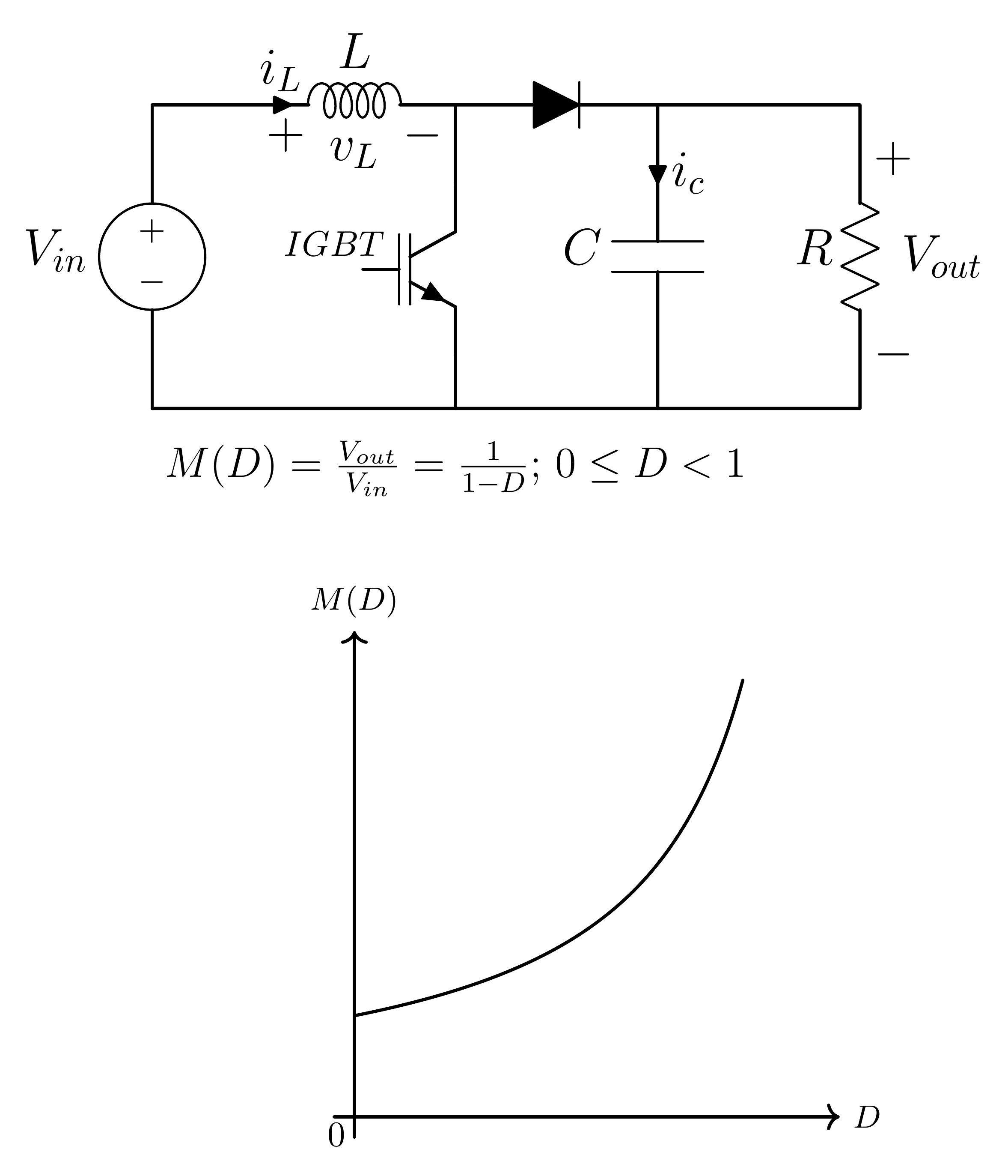
% Boost Converter
% This DC-DC converter increases the voltage level from input to output

% Designed by: Amir Ostadrahimi

\documentclass [border=5pt]{standalone}
\usepackage{tikz}
\usepackage[american,cuteinductors,smartlabels]{circuitikz} % A package to draw electrical networks with TikZ

%-- the dimensions of the elements can be changed here
\ctikzset{bipoles/thickness=0.7}
\ctikzset{bipoles/length=1.5cm}
\ctikzset{bipoles/resistor/width=.7}
\ctikzset{bipoles/resistor/height=.25}
\ctikzset{bipoles/diode/height=.3}
\ctikzset{bipoles/diode/width=.3}
\ctikzset{tripoles/thickness=.7}
\ctikzset{bipoles/vsourceam/height/.initial=.7}
\ctikzset{bipoles/vsourceam/width/.initial=.7}
\ctikzset{bipoles/vsourceam/width/.initial=.7}

%settings for fonts and lines
\tikzstyle{every node}=[font=\Large]
\tikzstyle{every path}=[line width=0.9 pt, line cap=round, line join=round]

\begin{document}

\begin{circuitikz}
%  Converter
\coordinate  (VBottom) at (0,0);
% VBottom stands for voltage source bottom and is located on (0,0)

\draw (VBottom) to [V, l=$V_{in}$, invert] ++(0,3) coordinate (VTop);
% "V" is to insert voltage source, instead of "V", you can use "battery", "battery1", and "battery2".
% the " l=$V_{in}$" is for label. You can use  "l_=$V_{in}$" or "l^=$V_{in}$" to change its location. 
%"invert" changes the polarity of the source. (VTop) stands for voltage top.

\draw (VTop) to [short] ++(1,0) to [L, l=$L$, v=$v_L$, i>^=$i_L$] ++(2,0) coordinate (InductorRight);
% "i>^=$i_L$ " is for showing the current of the element, by using "^" we can change its location and bring it at the input and the output of the element. By using  "<"  and  ">"  we can change its direction. And finally by using "_" we can change its vertical location.

\draw (InductorRight) to [short] ++(0,-0.8) node [nigbt, anchor=C, label={[xshift=-1.2cm, yshift=0] \normalsize $IGBT$}] (nigbt1){};
% here we used an N-channel IGBT using "nigbt". Alternatively, we could use "pigbt", "nmos", "pmos" and so on.

\draw (nigbt1.E) -- (nigbt1.E|-VBottom);
% using this command, a line starts from the Emitter of the IGBT and extends vertically until reaches the intersection of the vertical line from (nigbt1.E) and the horizontal line from (VB).

\draw (InductorRight) to [D*] ++(2,0) coordinate (DiodeRight) to [C, l_=$C$, i>^=$i_c$](DiodeRight|-VBottom);
% using [D*] makes the diode solid black. If we just use [D], the diode will be white.

\draw 
(DiodeRight) to [short] ++(2,0) coordinate(ResistorTop) to [R, l_=$R$, v^=$V_{out}$](ResistorTop|-VBottom) coordinate (ResistorBottom)

(ResistorBottom) -- (VBottom);

% Conversion Ratio
\coordinate [label={[xshift=0, yshift=0] \large $ M(D)=\frac{V_{out}}{V_{in}}=\frac{1}{1-D};$ \large $0 \leq D < 1$ }] (M) at (3,-1);

% Curve
\def\xo{2} % Axes of origin
\def\yo{-7} % Axes of origin
\def\length {5} % length of the axes
\def\N{200} %number of samples

\coordinate [label={[xshift=-5, yshift=-12] \normalsize$0$ }] (origin) at (\xo,\yo);

\draw[->] (\xo -0.2, \yo) -- ++(\length,0) node[right] {\small $D$};
\draw[->]  (\xo,\yo -0.2) -- ++(0, \length) node[above] {\small $M(D)$};
\draw plot[samples=\N, domain=0:0.77, xshift=\xo cm, yshift=\yo cm] (5*\x, {1/(1-\x)});

\end{circuitikz}

\end{document}

Summary

In these examples, we should note how to plot curves in the coordinate using TikZ syntax:

\draw plot[samples=\N, domain=0:4, xshift=\xo cm, yshift=\yo cm] (\x, \x);

\draw plot[samples=\N, domain=0:0.8, xshift=\xo cm, yshift=\yo cm] (5*\x, {-\x/(1-\x)});

\draw plot[samples=\N, domain=0:0.77, xshift=\xo cm, yshift=\yo cm] (5*\x, {1/(1-\x)});

Example 3: Half Wave Rectification

Example 3: Half Wave Rectification⁴

\documentclass[border=3pt]{standalone}
\usepackage[european,s traightvoltages, RPvoltages, americanresistor, americaninductors]{circuitikz}
\tikzset{every picture/.style={line width=0.2mm}}
\usepackage{amsmath}
\usetikzlibrary{calc}

\ctikzset{bipoles/thickness=1.2, label distance=1mm, voltage shift = 1}
\ctikzset{inductors/coils=4, inductors/width=1.2}
\ctikzset{quadpoles/transformer core/height=1.8}

\begin{document}
\begin{circuitikz}
%	%Grid
%	\def\length{6}
%	\draw[thin, dotted] (-\length,-\length) grid (\length,\length);
%	\foreach \i in {1,...,\length}
%	{
%		\node at (\i,-2ex) {\i};
%		\node at (-\i,-2ex) {-\i};	
%	}
%	\foreach \i in {1,...,\length}
%	{
%		\node at (-2ex,\i) {\i};	
%		\node at (-2ex,-\i) {-\i};	
%	}
%	\node at (-2ex,-2ex) {0};
	
	% Circuit
	\def\x{4}
	\def\y{3}
	\draw 
	(0,0) node[transformer core] (T) {}
	(T.B1) to [full diode, l=$D_1$] ++(\x,0) 
			to [R, l=$R$] ($(T.B2)+(\x,0)$) -- ++(-0.8*\x,0) 
			node[ground, pos=0.5] (ground) {} |- (T-L2.midtap);
			
	\draw[fill=black] (ground.north) circle (1.5pt);
\end{circuitikz}
\end{document}

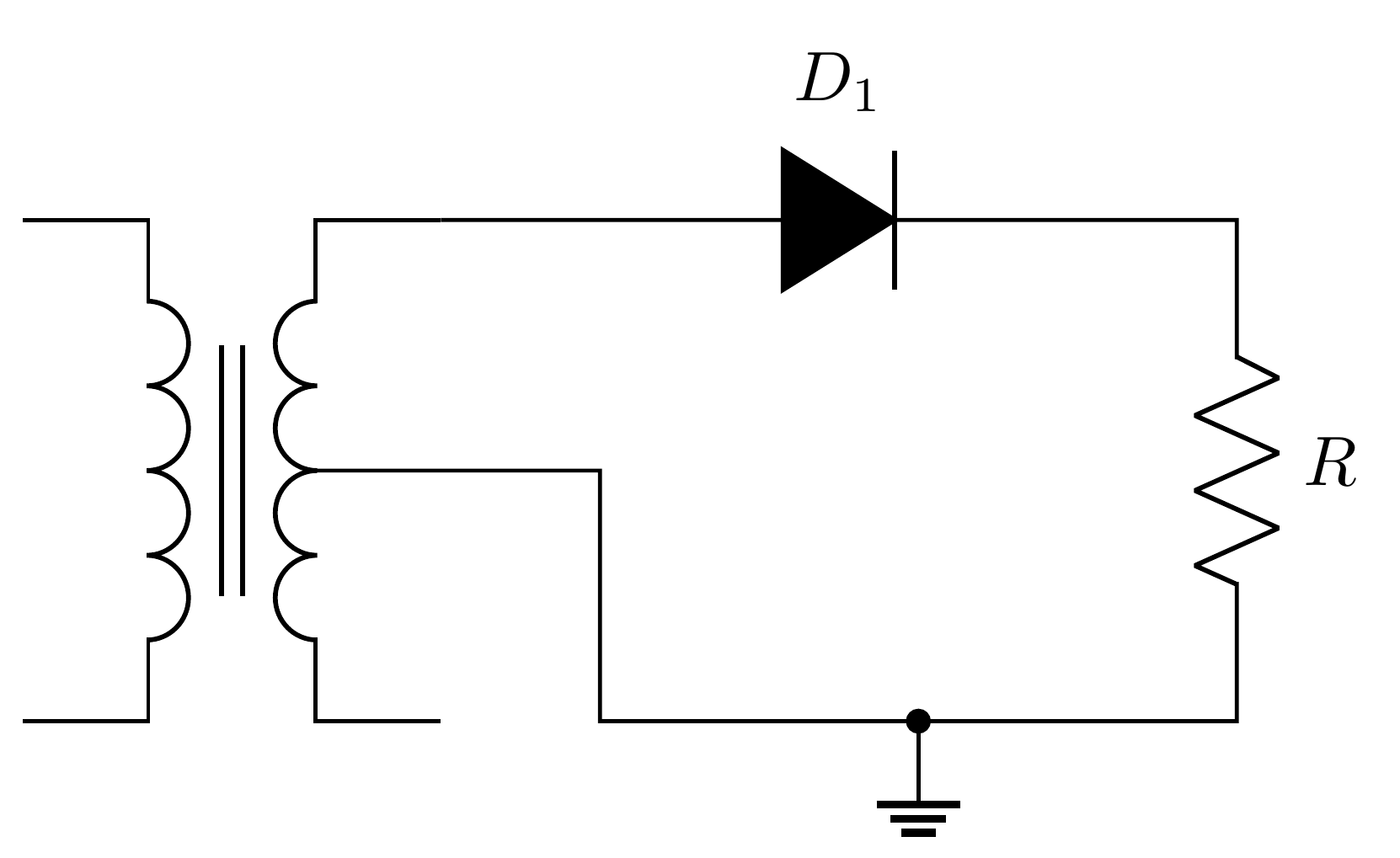
Well, the transformer is a very important component (or, device) in the fields of Electrical Engineering, and the CircuiTikZ also provides other styles of transformer (⁵, pp. 148-153).

Example 4: Basic Circuits

Example 4-1: AC circuits

Example 4-1: AC circuits⁶

% Author: Izaak Neutelings (Februari, 2020)
% http://texample.net/tikz/examples/tag/circuitikz/
% http://texample.net/tikz/examples/circuitikz/
% https://www.overleaf.com/learn/latex/CircuiTikz_package
% http://texdoc.net/texmf-dist/doc/latex/circuitikz/circuitikzmanual.pdf
% https://repositorios.cpai.unb.br/ctan/graphics/pgf/contrib/circuitikz/circuitikzmanual.pdf
\documentclass[border=3pt,tikz]{standalone}
\usepackage{amsmath} % for \dfrac
\usepackage{physics}
\usepackage{tikz,pgfplots}
\usepackage[siunitx]{circuitikz} %[symbols]
\usepackage[outline]{contour} % glow around text
\usetikzlibrary{arrows,arrows.meta}
\usetikzlibrary{decorations.markings}
\tikzset{>=latex} % for LaTeX arrow head
\usepackage{xcolor}
\colorlet{Icol}{blue!50!black}
\colorlet{Ccol}{orange!90!black}
\colorlet{Rcol}{green!50!black}
\colorlet{Lcol}{violet!90}
\colorlet{loopcol}{red!90!black!25}
\colorlet{pluscol}{red!60!black}
\colorlet{minuscol}{blue!60!black}
\newcommand\EMF{\mathcal{E}} %\varepsilon}
\contourlength{1.5pt}

%\tikzstyle{EMF}=[battery1,l=$\AC_0$,invert]
\tikzstyle{AC}=[sV,/tikz/circuitikz/bipoles/length=25pt,l=$\EMF(t)$]
\tikzstyle{internal R}=[R,color=Rcol,Rcol,l=$r$,/tikz/circuitikz/bipoles/length=30pt]
\tikzstyle{loop}=[->,red!90!black!25]
\tikzstyle{loop label}=[loopcol,fill=white,scale=0.8,inner sep=1]
\tikzstyle{thick R}=[R,color=Rcol,thick,Rcol,l=$R$]
\tikzstyle{thick C}=[C,thick,color=Ccol,Ccol,l=$C$]
\tikzstyle{thick L}=[L,thick,color=Lcol,Lcol,l=$L$,/tikz/circuitikz/bipoles/length=56pt] %inductor
\tikzstyle{thick Z}=[generic,color=Icol,thick,Icol,l=$Z$,fill=Icol!6]

\begin{document}
% AC, R
\begin{tikzpicture}
  \def\ang{155}
  \def\a{0.9}
  \def\b{0.8}
  \draw (0,0) to[AC] (0,2) --++(3,0)
              to[thick R] ++(0,-2) -- (0,0);
\end{tikzpicture}

% AC, C
\begin{tikzpicture}
  \def\ang{155}
  \def\a{0.9}
  \def\b{0.8}
  \draw (0,0) to[AC] (0,2) --++(3,0)
              to[thick C] ++(0,-2) -- (0,0);
  \node[minuscol,scale=0.8] at (2.55,0.55) {$-Q(t)$};
  \node[pluscol,scale=0.8] at (2.55,1.45) {$+Q(t)$};
\end{tikzpicture}

% AC, L
\begin{tikzpicture}
  \def\ang{155}
  \def\a{0.9}
  \def\b{0.8}
  \draw (0,0) to[AC] (0,2) --++(3,0)
              to[thick L] ++(0,-2) -- (0,0);
\end{tikzpicture}

% AC, RCL series
\begin{tikzpicture}
  \def\ang{120}
  \def\a{1.0}
  \def\b{0.8}
  \draw (0,0) to[AC] (0,2) to[thick R] ++(3,0)
              to[thick L] ++(0,-2) to[thick C] (0,0);
  \node[minuscol,scale=0.8] at (0.85,-0.25) {$-Q(t)$};
  \node[pluscol,scale=0.8] at (2.12,-0.25) {$+Q(t)$};
\end{tikzpicture}

% AC, RCL parallel
\begin{tikzpicture}
  \def\ang{155}
  \def\a{0.9}
  \def\b{0.8}
  \def\h{2.5}
  \def\w{1.8}
  \draw (0,0) to[AC] (0,\h) --
        (3*\w,\h) to[thick L] ++(0,-\h) -- (0,0)
        (1*\w,\h) to[thick R] ++(0,-\h)
        (2*\w,\h) to[thick C] ++(0,-\h);
  \draw[->,Icol] (0.88*\w,0.96*\h) --++ (0,-0.24*\h) node[midway,left=1] {$I_R$};
  \draw[->,Icol] (1.88*\w,0.96*\h) --++ (0,-0.24*\h) node[midway,left=1] {$I_C$};
  \draw[->,Icol] (2.88*\w,0.96*\h) --++ (0,-0.24*\h) node[midway,left=1] {$I_L$};
  \node[minuscol,scale=0.8,align=right] at (2.95,0.55) {$-Q(t)$};
  \node[pluscol,scale=0.8,align=right] at (2.95,1.45) {$+Q(t)$};
\end{tikzpicture}

% AC, RCL series
\begin{tikzpicture}
  \def\ang{120}
  \def\a{1.0}
  \def\b{0.8}
  \draw (0,0) to[AC] (0,2) --++(3,0)
              to[thick Z] ++(0,-2) -- (0,0);
\end{tikzpicture}

\end{document}

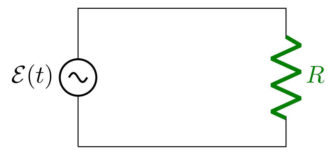
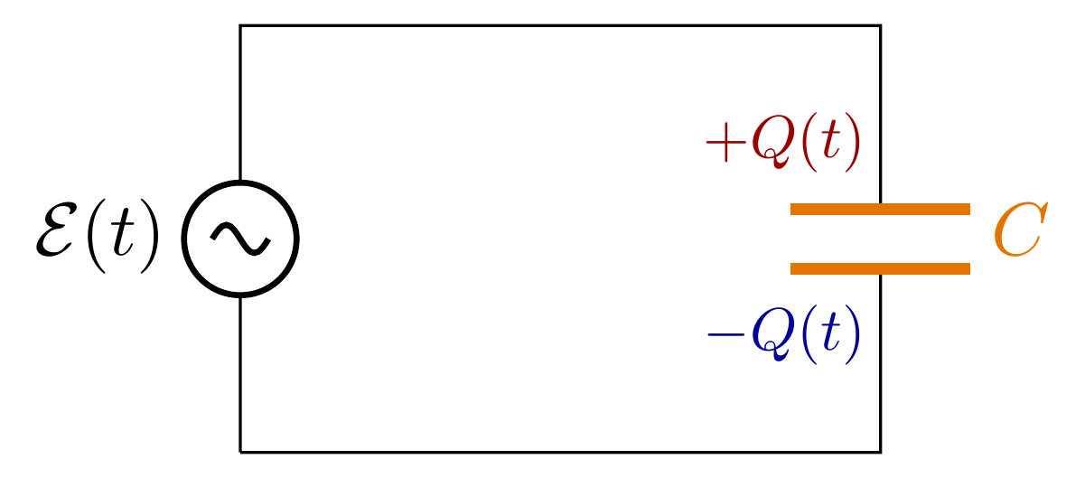
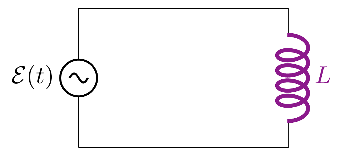
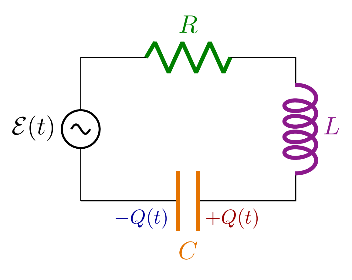
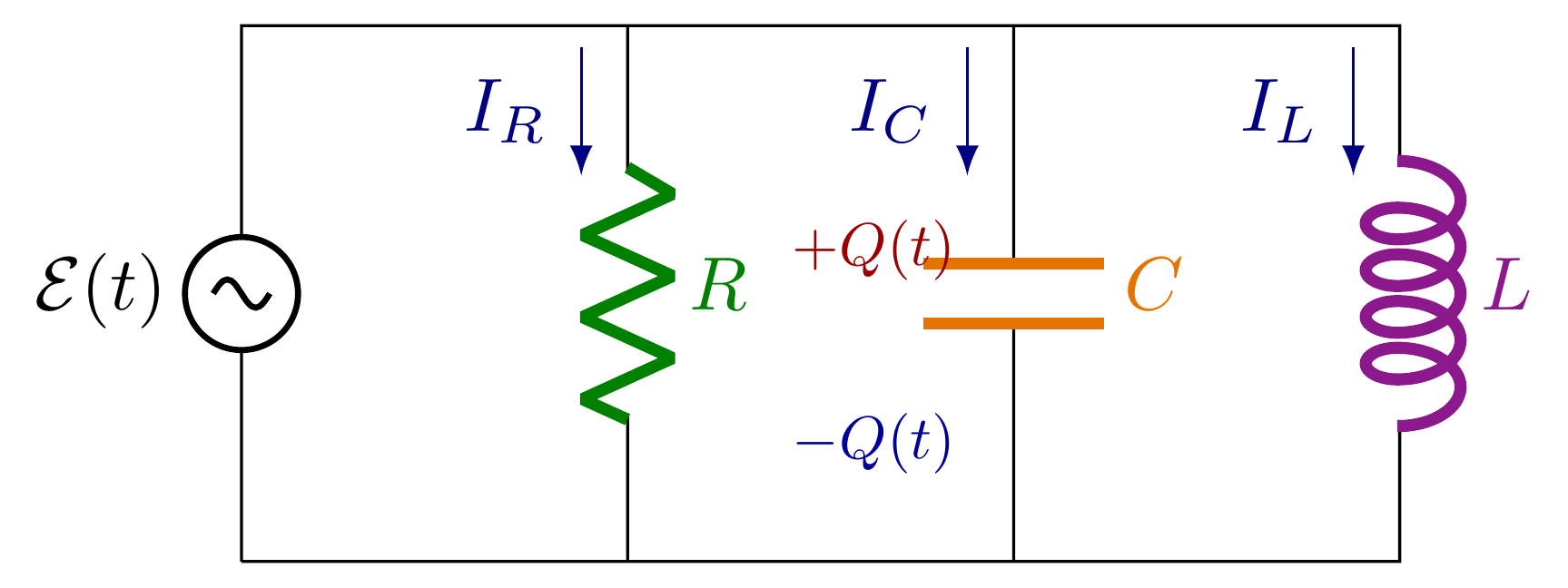
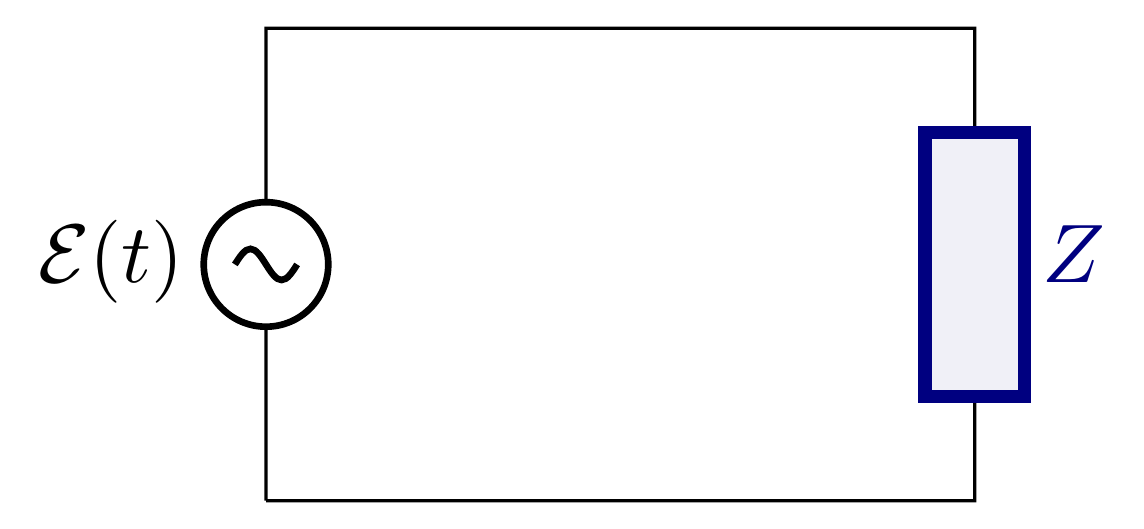
This example provides an easy way to customize components.

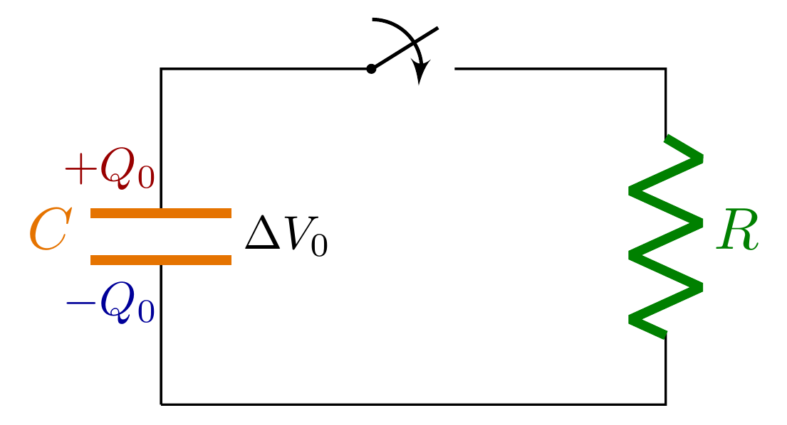
Example 4-2: RC circuit

Example 4-2: RC circuit⁷

% Author: Izaak Neutelings (Februari, 2020)
% http://texample.net/tikz/examples/tag/circuitikz/
% http://texample.net/tikz/examples/circuitikz/
% https://www.overleaf.com/learn/latex/CircuiTikz_package
% http://texdoc.net/texmf-dist/doc/latex/circuitikz/circuitikzmanual.pdf
% http://repositorios.cpai.unb.br/ctan/graphics/pgf/contrib/circuitikz/circuitikzmanual.pdf
\documentclass[border=3pt,tikz]{standalone}
\usepackage{amsmath} % for \dfrac
\usepackage{physics}
\usepackage{tikz,pgfplots}
\usepackage[siunitx]{circuitikz} %[symbols]
\usepackage[outline]{contour} % glow around text
\usetikzlibrary{arrows,arrows.meta}
\usetikzlibrary{decorations.markings}
\tikzset{>=latex} % for LaTeX arrow head
\usepackage{xcolor}
\colorlet{Icol}{blue!50!black}
\colorlet{Ccol}{orange!90!black}
\colorlet{Rcol}{green!50!black}
\colorlet{loopcol}{red!90!black!25}
\colorlet{pluscol}{red!60!black}
\colorlet{minuscol}{blue!60!black}
\newcommand\EMF{\mathcal{E}} %\varepsilon}
\contourlength{1.5pt}
\tikzstyle{EMF}=[battery1,l=$\EMF$,invert]
\tikzstyle{internal R}=[R,color=Rcol,Rcol,l=$r$,/tikz/circuitikz/bipoles/length=30pt]
\tikzstyle{loop}=[->,red!90!black!25]
\tikzstyle{loop label}=[loopcol,fill=white,scale=0.8,inner sep=1]
\tikzstyle{thick R}=[R,color=Rcol,thick,Rcol,l=$R$]
\tikzstyle{thick C}=[C,thick,color=Ccol,Ccol,l=$C$]
\tikzstyle{myswitch}=[closing switch,line width=0.3] %-{Latex[length=3]},

\newcommand{\myvoltmeter}[2] 
{  % #1 = name , #2 = rotation angle
  \begin{scope}[transform shape,rotate=#2]
  \draw[thick] (#1)node(){$\mathbf V$} circle (11pt);
  \draw[rotate=45,-latex] (#1)  +(-17pt,0) -- +(17pt,0);
  \end{scope}
}

\begin{document}
% RC with OPEN switch
\begin{tikzpicture}
  \def\ang{120}
  \def\a{1.0}
  \def\b{0.8}
  \draw (0,0) to[thick C] (0,2) to[myswitch] ++(3,0)
              to[thick R] ++(0,-2) -- (0,0);
  \fill[black] (1.25,2) circle (0.03);
  \node[minuscol,scale=0.8] at (-0.3,0.6) {$-Q_0$};
  \node[pluscol,scale=0.8] at (-0.3,1.4) {$+Q_0$};
  \node[scale=0.8] at (0.75,1) {$\Delta V_0$};
\end{tikzpicture}

% RC with CLOSED switch
\begin{tikzpicture}
  \def\ang{120}
  \def\a{1.0}
  \def\b{0.8}
  \draw (0,0) to[thick C] (0,2) -- ++(3,0)
              to[thick R] ++(0,-2) -- (0,0);
  \fill[black] (1.25,2) circle (0.03);
  \draw[line width=0.6] (1.25,2) -- ++(0.48,0); % Closed switch
  \node[minuscol,scale=0.8] at (-0.3,0.6) {$-Q$};
  \node[pluscol,scale=0.8] at (-0.3,1.4) {$+Q$};
  \node[scale=0.8] at (0.75,1) {$\Delta V$};
  \draw[->,Icol] ({1.5+\a*cos(\ang)},{1+\b*sin(\ang)}) arc (\ang:-120:{\a} and {\b})
                 node[midway,left=3,scale=0.9] {$I$};
\end{tikzpicture}

% RC+EMF with OPEN switch
\begin{tikzpicture}
  \def\ang{120}
  \def\a{1.0}
  \def\b{0.8}
  \draw (0,0) to[EMF] (0,2) to[myswitch] ++(3,0)
              to[thick R] ++(0,-2) to[thick C] (0,0);
  \fill[black] (1.25,2) circle (0.03);
  \node at (-0.35,0.7) {$-$};
  \node at (-0.35,1.4) {$+$};
\end{tikzpicture}

% RC+EMF with CLOSED switch
\begin{tikzpicture}
  \def\ang{220}
  \def\a{0.9}
  \def\b{0.8}
  \draw[->,Icol] ({1.5+\a*cos(\ang)},{1+\b*sin(\ang)}) arc (\ang:-40:{\a} and {\b})
                 node[midway,below=3,scale=0.9] {$I$};
  \draw (0,0) to[EMF] (0,2) -- ++(3,0)
              to[thick R] ++(0,-2) to[thick C] (0,0);
  \fill[black] (1.25,2) circle (0.03);
  \draw[line width=0.6] (1.25,2) -- ++(0.48,0);
  \node at (-0.35,0.7) {$-$};
  \node at (-0.35,1.4) {$+$};
  \node[minuscol,scale=0.8] at (1.0,-0.25) {$-Q$};
  \node[pluscol,scale=0.8] at (1.98,-0.25) {$+Q$};
  \node[scale=0.8] at (1.5,0.6) {$\Delta V$};
\end{tikzpicture}

\end{document}

Note the way of drawing the curved arrow:

\draw[->,Icol] ({1.5+\a*cos(\ang)},{1+\b*sin(\ang)}) arc (\ang:-40:{\a} and {\b})
               node[midway,below=3,scale=0.9] {$I$};

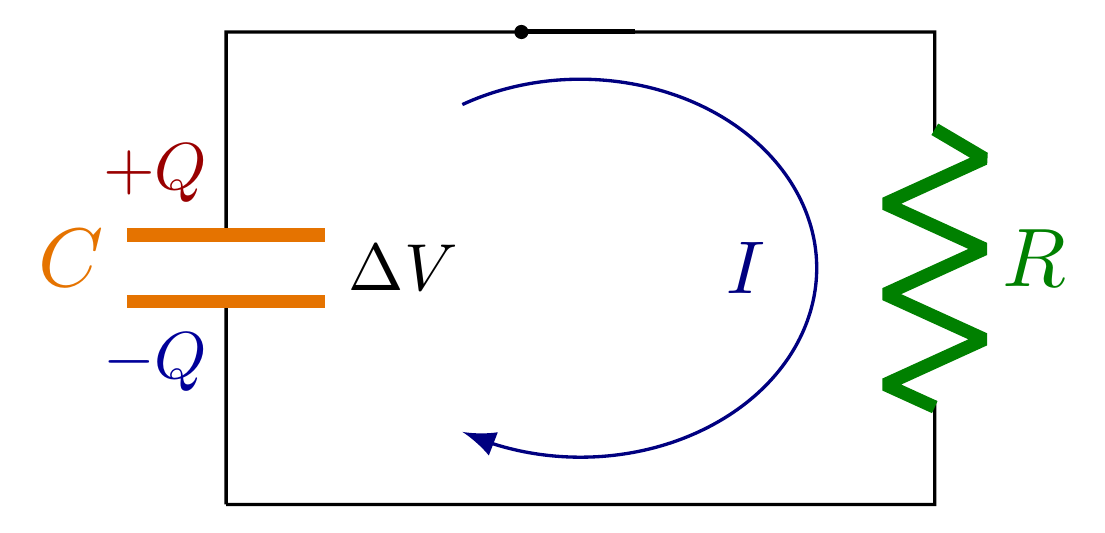
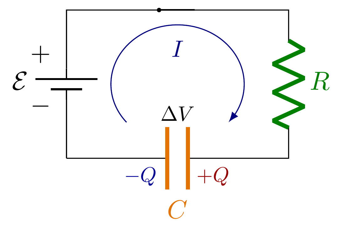
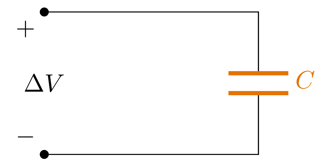
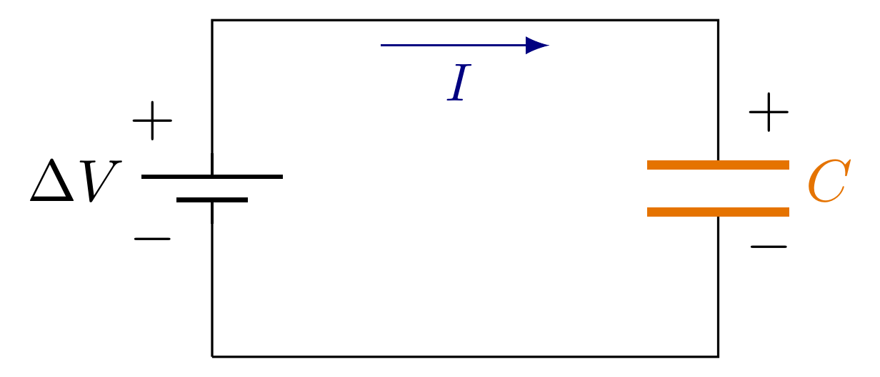
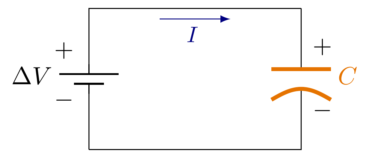
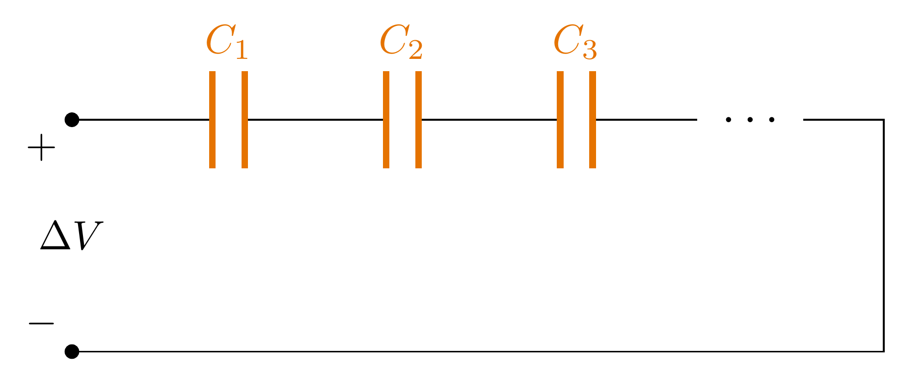
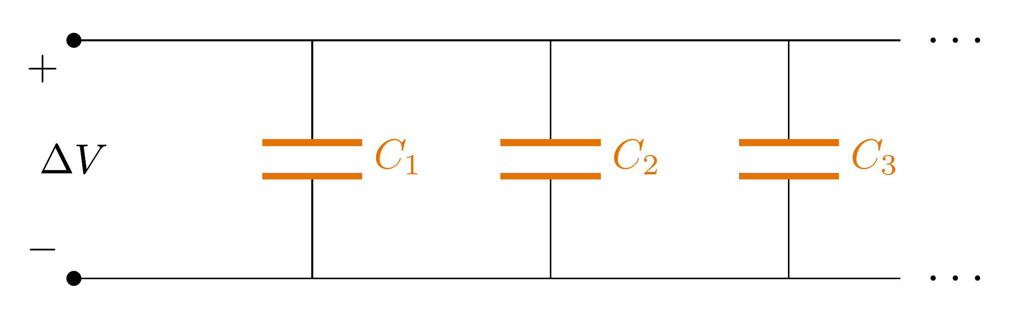
Example 4-3: Circuit with capacitors

Example 4-3: Circuit with capacitors⁸

% Author: Izaak Neutelings (Februari, 2020)
% http://texample.net/tikz/examples/tag/circuitikz/
% http://texample.net/tikz/examples/circuitikz/
% https://www.overleaf.com/learn/latex/CircuiTikz_package
% http://texdoc.net/texmf-dist/doc/latex/circuitikz/circuitikzmanual.pdf
% http://repositorios.cpai.unb.br/ctan/graphics/pgf/contrib/circuitikz/circuitikzmanual.pdf
\documentclass[border=3pt,tikz]{standalone}
\usepackage{amsmath} % for \dfrac
\usepackage{physics}
\usepackage{tikz,pgfplots}
\usepackage[siunitx]{circuitikz} %[symbols]
\usepackage{xcolor}
\tikzset{>=latex} % for LaTeX arrow head
\colorlet{Icol}{blue!50!black}
\colorlet{Ccol}{orange!90!black}
\colorlet{pluscol}{red!60!black}
\colorlet{minuscol}{blue!60!black}
%\tikzstyle{charged}=[top color=blue!20,bottom color=blue!40,shading angle=10]
\tikzstyle{thick C}=[C,thick,color=Ccol,Ccol,l=$C$]
\tikzstyle{mybattery}=[battery1,l=$\Delta V$,invert]

\begin{document}
% CAPACITOR without battery
\begin{tikzpicture}
  \draw (0,2) to [short,*-] (3,2) to[thick C] (3,0) to [short,-*] (0,0);
  \node[below left] at (0,2) {$+$};
  \node[above left] at (0,0) {$-$};
  \node at (0,1) {$\Delta V$};
\end{tikzpicture}

% CAPACITOR with battery
\begin{tikzpicture}
  \draw (0,0) to[mybattery] (0,2) -- (3,2)
              to[thick C] (3,0) -- (0,0);
  \node at (-0.35,0.7) {$-$};
  \node at (-0.35,1.4) {$+$};
  \node at (3.3,0.65) {$-$};
  \node at (3.3,1.45) {$+$};
  \draw[->,Icol] (1.0,1.85) --++ (1,0)
                 node[midway,left=1,below,scale=0.9] {$I$};
\end{tikzpicture}

% POLARIZED CAPACITOR with battery
\begin{tikzpicture}
  \draw (0,0) to[mybattery] (0,2) -- (3,2)
        (0,0) -- (3,0) to[polar capacitor,color=Ccol,thick,Ccol,l_=$C$] (3,2);
              %to[polar capacitor,color=Ccol,thick,l=$C$,reverse] (3,0) -- (0,0);
  \node at (-0.35,0.7) {$-$};
  \node at (-0.35,1.4) {$+$};
  \node at (3.3,0.55) {$-$};
  \node at (3.3,1.45) {$+$};
  %\node at (3.7,0.95) {$C$};
  \draw[->,Icol] (1.0,1.85) --++ (1,0)
                 node[midway,left=1,below,scale=0.9] {$I$};
\end{tikzpicture}

% POLARIZED CAPACITOR with battery
\begin{tikzpicture}
  \draw (0,0) to[polar capacitor,color=Ccol,thick,Ccol,l_=$C$] (0,2);
  \node at (0.3,0.55) {$-$};
  \node at (0.3,1.45) {$+$};
\end{tikzpicture}

% CAPACITORS in series
\begin{tikzpicture}
  \draw (0,2) to [short,*-] (0.6,2)
              to[thick C,l=$C_1$] ++(1.5,0)
              to[thick C,l=$C_2$] ++(1.5,0)
              to[thick C,l=$C_3$] ++(1.5,0)
              %(6,2) to[C,color=Ccol,thick,l=$C_4$]
              -- ++(1.5,0) node[midway,fill=white,inner sep=5,scale=1.2] {$.\,.\,.$}
              -- (7,2) -- (7,0) to[short,-*] (0,0);
  \node at (0,1) {$\Delta V$};
  \node[below left] at (0,2) {$+$};
  \node[above left] at (0,0) {$-$};
\end{tikzpicture}

% CAPACITORS in parallel
\begin{tikzpicture}
  \node[fill=white,inner sep=5,scale=1.2] (ET) at (7.4,2) {$.\,.\,.$};
  \node[fill=white,inner sep=5,scale=1.2] (EB) at (7.4,0) {$.\,.\,.$};
  \node at (0,1) {$\Delta V$};
  %\draw (0,0) to[battery1] (0,2) -- (2,2) to[C,color=Ccol,thick,l=$C_1$] (2,0) -- (0,0);
  \draw (0,2) to[short,*-] (2,2) to[thick C,l=$C_1$] (2,0) to[short,-*] (0,0);
  \draw (2,2) -- (4,2) to[thick C,l=$C_2$] (4,0) -- (2,0);
  \draw (4,2) -- (6,2) to[thick C,l=$C_3$] (6,0) -- (4,0);
  \draw (6,2) -- (ET.180);
  \draw (6,0) -- (EB.180);
  %\draw (6,2) -- (8,2) to[C,color=Ccol,thick,l=$C_4$] (8,0) -- (6,0);
  \node at (0,1) {$\Delta V$};
  \node[below left] at (0,2) {$+$};
  \node[above left] at (0,0) {$-$};
\end{tikzpicture}

\end{document}

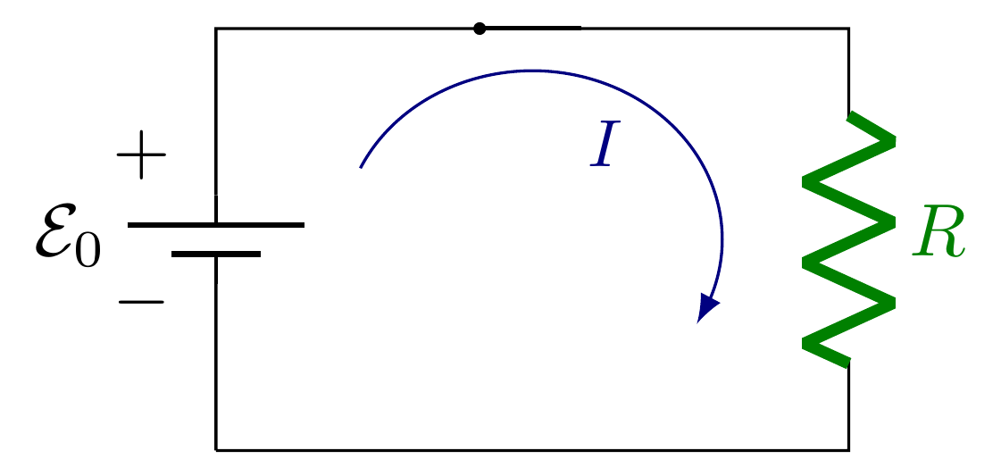
Example 4-4: RLC circuit (DC)

Example 4-4: RLC circuit (DC)⁹

% Author: Izaak Neutelings (Februari, 2020)
% http://texample.net/tikz/examples/tag/circuitikz/
% http://texample.net/tikz/examples/circuitikz/
% https://www.overleaf.com/learn/latex/CircuiTikz_package
% http://texdoc.net/texmf-dist/doc/latex/circuitikz/circuitikzmanual.pdf
% http://repositorios.cpai.unb.br/ctan/graphics/pgf/contrib/circuitikz/circuitikzmanual.pdf
\documentclass[border=3pt,tikz]{standalone}
\usepackage{amsmath} % for \dfrac
\usepackage{physics}
\usepackage{tikz,pgfplots}
\usepackage[siunitx]{circuitikz} %[symbols]
\usepackage[outline]{contour} % glow around text
\usetikzlibrary{arrows,arrows.meta}
\usetikzlibrary{decorations.markings}
\tikzset{>=latex} % for LaTeX arrow head
\usepackage{xcolor}
\colorlet{Icol}{blue!50!black}
\colorlet{Ccol}{orange!90!black}
\colorlet{Rcol}{green!50!black}
\colorlet{Lcol}{violet!90}
\colorlet{loopcol}{red!90!black!25}
\colorlet{pluscol}{red!60!black}
\colorlet{minuscol}{blue!60!black}
\newcommand\EMF{\mathcal{E}} %\varepsilon}
\contourlength{1.5pt}
\tikzstyle{EMF}=[battery1,l=$\EMF_0$,invert]
\tikzstyle{internal R}=[R,color=Rcol,Rcol,l=$r$,/tikz/circuitikz/bipoles/length=30pt]
\tikzstyle{loop}=[->,red!90!black!25]
\tikzstyle{loop label}=[loopcol,fill=white,scale=0.8,inner sep=1]
\tikzstyle{thick R}=[R,color=Rcol,thick,Rcol,l=$R$]
\tikzstyle{thick C}=[C,thick,color=Ccol,Ccol,l=$C$]
\tikzstyle{thick L}=[L,thick,color=Lcol,Lcol,l=$L$,/tikz/circuitikz/bipoles/length=56pt] %inductor
\tikzstyle{myswitch}=[closing switch,line width=0.3] %-{Latex[length=3]}
\newcommand{\closedswitch}[1]{
  \draw[line width=0.6] (#1) --++ (0.48,0);
  \fill[black] (#1) circle (0.03);
}

\newcommand{\myvoltmeter}[2] 
{  % #1 = name , #2 = rotation angle
  \begin{scope}[transform shape,rotate=#2]
  \draw[thick] (#1)node(){$\mathbf V$} circle (11pt);
  \draw[rotate=45,-latex] (#1)  +(-17pt,0) --+(17pt,0);
  \end{scope}
}

\begin{document}
% R with CLOSED switch
\begin{tikzpicture}
  \def\ang{155}
  \def\a{0.9}
  \def\b{0.8}
  \draw[->,Icol] ({1.5+\a*cos(\ang)},{1+\b*sin(\ang)}) arc (\ang:-30:{\a} and {\b})
                 node[midway,left=2,below=1,scale=0.9] {$I$};
  \draw (0,0) to[EMF] (0,2) --++(3,0)
              to[thick R] ++(0,-2) -- (0,0);
  \closedswitch{1.25,2};
  \node at (-0.35,0.7) {$-$};
  \node at (-0.35,1.4) {$+$};
\end{tikzpicture}

% RL with CLOSED switch
\begin{tikzpicture}
  \def\ang{155}
  \def\a{1.0}
  \def\b{0.8}
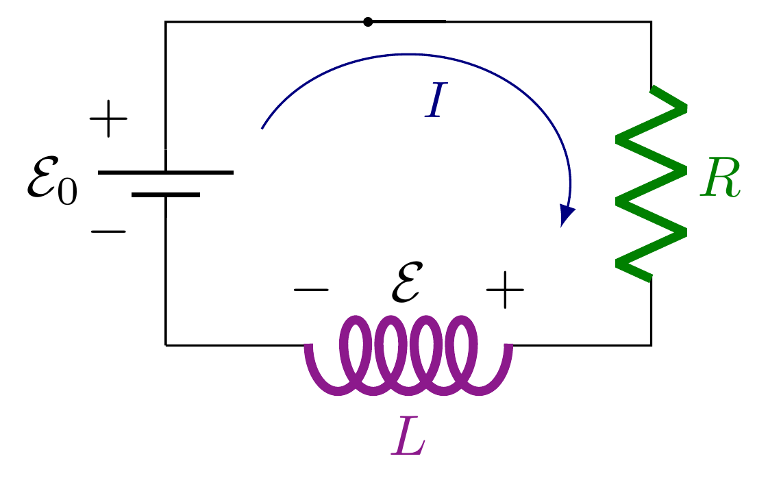
  \draw (0,0) to[EMF] (0,2) --++(3,0) %to[myswitch]
              to[thick R] ++(0,-2) to[thick L] (0,0);
  \draw[->,Icol] ({1.5+\a*cos(\ang)},{1+\b*sin(\ang)}) arc (\ang:-20:{\a} and {\b})
                 node[midway,left=6,below=0,scale=0.9] {$I$};
  \closedswitch{1.25,2};
  \node at (-0.35,0.7) {$-$};
  \node at (-0.35,1.4) {$+$};
  \node at (0.90,0.34) {$-$};
  \node at (2.10,0.34) {$+$};
  \node at (1.50,0.39) {$\EMF$};
\end{tikzpicture}

% RC with OPEN switch
\begin{tikzpicture}
  \def\ang{120}
  \def\a{1.0}
  \def\b{0.8}
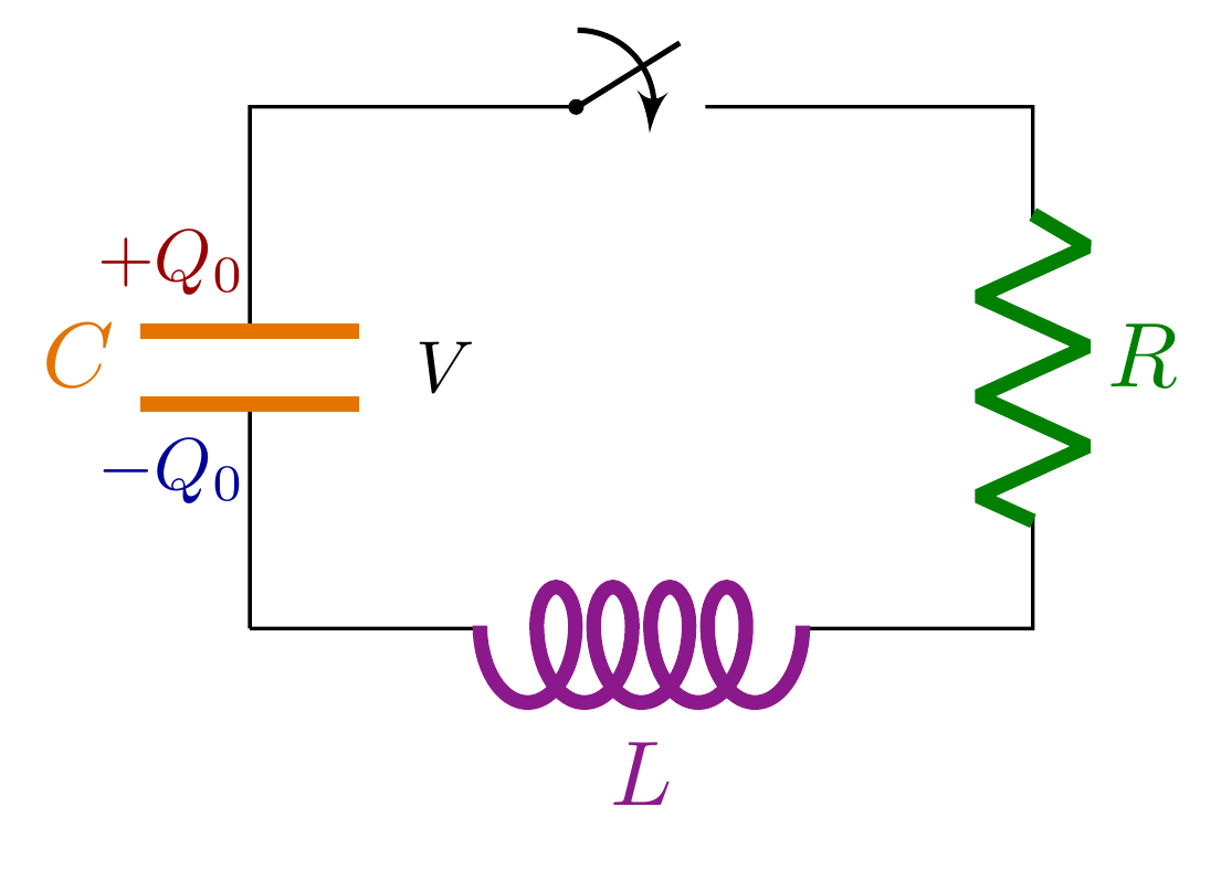
  \draw (0,0) to[thick C] (0,2) to[myswitch] ++(3,0)
              to[thick L] ++(0,-2) -- (0,0);
  \fill[black] (1.25,2) circle (0.03);
  \node[minuscol,scale=0.8] at (-0.3,0.6) {$-Q_0$};
  \node[pluscol,scale=0.8] at (-0.3,1.4) {$+Q_0$};
  \node[scale=0.8] at (0.75,1) {$V$};
\end{tikzpicture}

% RCL with OPEN switch
\begin{tikzpicture}
  \def\ang{120}
  \def\a{1.0}
  \def\b{0.8}
  \draw (0,0) to[thick C] (0,2) to[myswitch] ++(3,0)
              to[thick R] ++(0,-2) to[thick L] (0,0);
  \fill[black] (1.25,2) circle (0.03);
  \node[minuscol,scale=0.8] at (-0.3,0.6) {$-Q_0$};
  \node[pluscol,scale=0.8] at (-0.3,1.4) {$+Q_0$};
  \node[scale=0.8] at (0.75,1) {$V$};
\end{tikzpicture}

\end{document}

References