Karush–Kuhn–Tucker Conditions (KKT Conditions)
KKT conditions
The method of Lagrange multipliers is used to solve an optimization with equality constraints, by converting the equality-constrained problem into an unconstrained problem1. When there are inequalities in the optimization problem, analogous to the Lagrange function, we can construct a generalized Lagrange function, and correspondingly we’ll have Karush–Kuhn–Tucker (KKT) conditions2:
In mathematical optimization, the Karush–Kuhn–Tucker (KKT) conditions, also known as the Kuhn–Tucker conditions, are first derivative tests (sometimes called first-order necessary conditions) for a solution in nonlinear programming to be optimal, provided that some regularity conditions are satisfied.
Allowing inequality constraints, the KKT approach to nonlinear programming generalizes the method of Lagrange multipliers, which allows only equality constraints. Similar to the Lagrange approach, the constrained maximization (minimization) problem is rewritten as a Lagrange function whose optimal point is a global maximum or minimum over the domain of the choice variables and a global minimum (maximum) over the multipliers. The Karush–Kuhn–Tucker theorem is sometimes referred to as the saddle-point theorem.
Compared with the method of Lagrange multipliers, the KKT approach takes inequalities into consideration. To figure out what are KKT conditions and why they work, we should ask, as we did when deriving the method of Lagrange method1, which kinds of characteristics will the optimal points have when there exist inequalities in the optimization problem? For the convenience of discussion, we can firstly consider a bivariate minimization problem with one inequality:
\[\begin{split} \min_{\boldsymbol{\mathrm{x}}}\ &f(\boldsymbol{\mathrm{x}})\\ \text{s.t.}\ &g(\boldsymbol{\mathrm{x}})\le0\\ \end{split}\]where $\boldsymbol{\mathrm{x}}\in\mathbb{R}^2$. Let \(\boldsymbol{\mathrm{x}}^*\) denotes the optimal points, i.e., \(f(\boldsymbol{\mathrm{x}}^*)\) is a minimum, there are two possible cases for \(\boldsymbol{\mathrm{x}}^*\):
Case 1: \(g(\boldsymbol{\mathrm{x}}^*)<0\), i.e. the inequality constraint is strictly satisfied, or rather, the inequality is not active at points \(\boldsymbol{\mathrm{x}}^*\).
For the univariate case3:
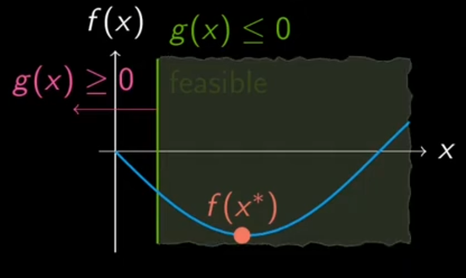
In this case, there is:
\[g(\boldsymbol{\mathrm{x}}^*)<0\label{eq4}\]and because $\boldsymbol{\mathrm{x}}^*$ is optimal, we have:
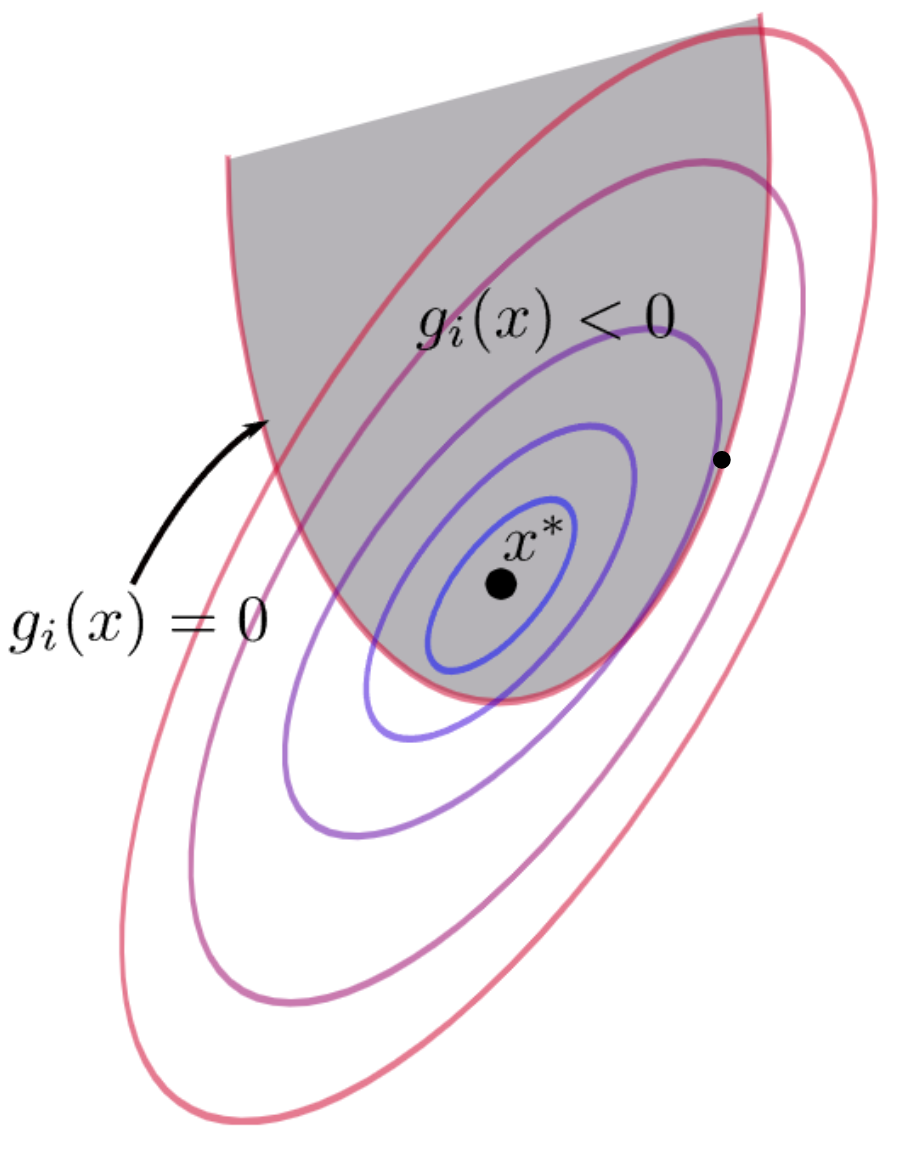
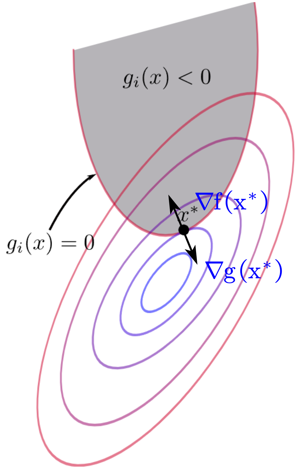
\[\nabla f(\boldsymbol{\mathrm{x}}^*)=\boldsymbol{\mathrm{0}}\label{eq1}\]Case 2: \(g(\boldsymbol{\mathrm{x}}^*)=0\), i.e., the inequality is active at points \(\boldsymbol{\mathrm{x}}^*\).
Similarly, for the univariate case:
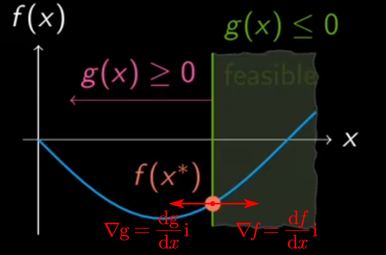
As can be seen from the figure, \(\boldsymbol{\mathrm{x}}^*\) locates at the boundary of area where \(g(\boldsymbol{\mathrm{x}}^*)\le0\) (i.e., gray area in the figure). Because \(\nabla g\) points towards the direction where \(g\) increases, $\nabla g(\boldsymbol{\mathrm{x}}^*)$ points towards the outside of the gray area (since points \(\boldsymbol{\mathrm{x}}\) in the area satisfy \(g(\boldsymbol{\mathrm{x}})<0\), whereas \(\boldsymbol{\mathrm{x}}\) out of the area satisfy \(g(\boldsymbol{\mathrm{x}})>0\)). On the other hand, because \(\nabla f\) points towards the the direction where $f$ increases and \(\boldsymbol{\mathrm{x}}^*\) is a minimum, we have $\nabla f(\boldsymbol{\mathrm{x}}^*)$ points towards to the inside of the gray area (since if \(\nabla f(\boldsymbol{\mathrm{x}}^\ast)\) points towards to the outside of the area, $f$ will further decreases along the direction inside of the area, then \(\boldsymbol{\mathrm{x}}^*\) can’t stay at the boundary of area). Finally, we can conclude that, $\nabla g(\boldsymbol{\mathrm{x}}^\ast)$ and $\nabla f(\boldsymbol{\mathrm{x}}^\ast)$ are parallel (because $f$ and $g$ are tangent at $\boldsymbol{\mathrm{x}}^\ast$) and they are in an opposite direction, that is:
\[\nabla f(\boldsymbol{\mathrm{x}}^*)+\lambda\nabla g(\boldsymbol{\mathrm{x}}^*)=\boldsymbol{\mathrm{0}}\label{eq6}\]where:
\[\lambda>0\label{eq7}\]and of course the constraint:
\[g(\boldsymbol{\mathrm{x}}^*)=0\label{eq8}\]To include both cases, we can firstly rewrite $\eqref{eq1}$ as:
\[\left\{ \begin{split} & \nabla f(\boldsymbol{\mathrm{x}}^*)+\lambda\nabla g(\boldsymbol{\mathrm{x}}^*)=\boldsymbol{\mathrm{0}}\\ & \lambda=0 \end{split}\right.\label{eq5}\]Then, for the first case, $\eqref{eq4}$ and $\eqref{eq5}$, we have:
\[\left\{ \begin{split} & g(\boldsymbol{\mathrm{x}}^*)<0\\ & \nabla f(\boldsymbol{\mathrm{x}}^*)+\lambda\nabla g(\boldsymbol{\mathrm{x}}^*)=\boldsymbol{\mathrm{0}}\\ & \lambda=0 \end{split}\right.\label{eq2}\]and for the second one, $\eqref{eq6}$, $\eqref{eq7}$, and $\eqref{eq8}$:
\[\left\{ \begin{split} & g(\boldsymbol{\mathrm{x}}^*)=0\\ & \nabla f(\boldsymbol{\mathrm{x}}^*)+\lambda\nabla g(\boldsymbol{\mathrm{x}}^*)=\boldsymbol{\mathrm{0}}\\ & \lambda>0 \end{split}\right.\label{eq3}\]Finally, combine $\eqref{eq2}$ and $\eqref{eq3}$, we’ll have:
\[\left\{ \begin{split} &g(\boldsymbol{\mathrm{x}})\le0\ \text{is not active} \left\{ \begin{split} & g(\boldsymbol{\mathrm{x}}^*)<0\\ & \nabla f(\boldsymbol{\mathrm{x}}^*)+\lambda\nabla g(\boldsymbol{\mathrm{x}}^*)=\boldsymbol{\mathrm{0}}\\ & \lambda=0\\ \end{split}\right.\\ &g(\boldsymbol{\mathrm{x}})\le0\ \text{is active} \left\{ \begin{split} & g(\boldsymbol{\mathrm{x}}^*)=0\\ & \nabla f(\boldsymbol{\mathrm{x}}^*)+\lambda\nabla g(\boldsymbol{\mathrm{x}}^*)=\boldsymbol{\mathrm{0}}\\ & \lambda>0\\ \end{split}\right. \end{split}\right.\notag\]Incorporate these two sets of constraints, we’ll have:
\[\left\{ \begin{split} & \nabla f(\boldsymbol{\mathrm{x}}^*)+\lambda\nabla g(\boldsymbol{\mathrm{x}}^*)=\boldsymbol{\mathrm{0}}\\ & g(\boldsymbol{\mathrm{x}}^*)\le0\\ & \lambda\ge0\\ & \lambda g(\boldsymbol{\mathrm{x}}^*)=0\\ \end{split}\right.\label{eq9}\]where \(\lambda g(\boldsymbol{\mathrm{x}}^*)=0\) holds because for the first case, \(g(\boldsymbol{\mathrm{x}}^*)<0\) and \(\lambda=0\), and for the second case, \(g(\boldsymbol{\mathrm{x}}^*)=0\) and \(\lambda>0\).
So, we could conclude that, when $\boldsymbol{\mathrm{x}}^*$ is an optimal point, then conditions $\eqref{eq9}$ are satisfied, and these conditions $\eqref{eq9}$ are called KKT conditions. Among which3:
- \(\nabla f(\boldsymbol{\mathrm{x}}^*)+\lambda\nabla g(\boldsymbol{\mathrm{x}}^*)=\boldsymbol{\mathrm{0}}\) is the stationarity condition, sometimes denoted as KKT14
- $g(\boldsymbol{\mathrm{x}}^*)\le0$ is the primal feasibility
- $\lambda\ge0$ is the dual feasibility, because $\lambda$ is also called as dual variables5
- $\lambda g(\boldsymbol{\mathrm{x}}^*)=0$ is the complementary slackness (or complementarity conditions), sometimes denoted as KKT24
Although in the above text, we take a bivariate case with one-inequality to derive KKT conditions $\eqref{eq9}$, they are also available for the multi-variate case and when there are multiple inequality constraints and multiple equality constraints (by combining the method of Lagrange multipliers1). Here is a relatively complete definition6:
Suppose $\boldsymbol{\mathrm{x}}^*$ is a local minimum point of an inequality constrained problem:
\[\begin{split} \min_{\boldsymbol{\mathrm{x}}}\ &f(\boldsymbol{\mathrm{x}})\\ \text{s.t.}\ &h_i(\boldsymbol{\mathrm{x}})\le0,\ i=1,\cdots,l\\ \ &g_i(\boldsymbol{\mathrm{x}})=0,\ i=1,\cdots,m\\ \end{split}\]If $\boldsymbol{\mathrm{x}}^\ast$ is regular for all equality constraints and active inequality constraints, then there exists Lagrange/KKT multipliers $\lambda_1^\ast,\cdots,\lambda_m^\ast,\mu_1^\ast,\cdots,\mu_l^\ast$ such that:
\[\nabla f(\boldsymbol{\mathrm{x}}^*)+\sum_{i=1}^m\lambda_i^*\nabla g_i(\boldsymbol{\mathrm{x}}^*)+\sum_{i=1}^l\mu_i^*\nabla h_i(\boldsymbol{\mathrm{x}}^*)=\boldsymbol{\mathrm{0}}\] \[\mu_i^*h_i(\boldsymbol{\mathrm{x}}^*)=0,\ i=1,\cdots,l\] \[\mu_i\ge0,\ i=1,\cdots,l\] \[h_i(\boldsymbol{\mathrm{x}}^*)\le0,\ i=1,\cdots,l\] \[g_i(\boldsymbol{\mathrm{x}}^*)=0,\ i=1,\cdots,m\]By the way, as can be seen, unlike the method of Lagrange multipliers, when there are inequalities we can’t get an unconstrained optimization problem by a certain of conversion — some inequality constraints always exist.
Analogous to the method of Lagrange function, we can construct an auxiliary function, i.e., the generalized Lagrangian5:
\[\mathcal{L}(\boldsymbol{\mathrm{x}},\boldsymbol{\mathrm{\lambda}},\boldsymbol{\mathrm{\mu}})\equiv f(\boldsymbol{\mathrm{x}})+\sum_{i=1}^m\lambda_ig_i(\boldsymbol{\mathrm{x}})+\sum_{i=1}^l\mu_ih_i(\boldsymbol{\mathrm{x}})\]where $(\boldsymbol{\mathrm{\lambda}},\boldsymbol{\mathrm{\mu}})\in\mathbb{R}^l\times\mathbb{R}^m_+$, then we’ll have KKT conditions as the form:
\[\nabla_{\boldsymbol{\mathrm{x}}}\mathcal{L}(\boldsymbol{\mathrm{x}},\boldsymbol{\mathrm{\lambda}},\boldsymbol{\mathrm{\mu}})=\boldsymbol{0}\] \[\nabla_{\boldsymbol{\mathrm{\lambda}}}\mathcal{L}(\boldsymbol{\mathrm{x}},\boldsymbol{\mathrm{\lambda}},\boldsymbol{\mathrm{\mu}})=\boldsymbol{\mathrm{0}}\] \[\boldsymbol{\mathrm{h}}(\boldsymbol{\mathrm{x}})\le\boldsymbol{\mathrm{0}}\] \[\boldsymbol{\mathrm{\mu}}\ge\boldsymbol{\mathrm{0}}\] \[\boldsymbol{\mathrm{\mu}}\odot\boldsymbol{\mathrm{h}}(\boldsymbol{\mathrm{x}})=\boldsymbol{\mathrm{0}}\]Examples
Example 1
Consider the minimization6:
\[\begin{split} \min\ &x_1^2+x_2^2\\ \text{s.t.}\ &x_1+x_2=1\\ \ &x_2\le\alpha\\ \end{split}\]The KKT conditions are:
\[\left\{\begin{split} &\nabla_{\boldsymbol{\mathrm{x}}}(x_1^2+x_2^2)+\lambda\nabla_{\boldsymbol{\mathrm{x}}}(x_1+x_2-1)+\mu\nabla_{\boldsymbol{\mathrm{x}}}(x_2-\alpha)=0\\ &x_1+x_2-1=0\\ &x_2\le\alpha\\ &\mu\ge0\\ &\mu(x_2-\alpha)=0\\ \end{split}\right.\]i.e.
\[\left\{\begin{split} &2x_1+\lambda=0\\ &2x_2+\lambda+\mu=0\\ &x_1+x_2-1=0\\ &x_2\le\alpha\\ &\mu\ge0\\ &\mu(x_2-\alpha)=0\\ \end{split}\right.\](1) When $\mu=0$, that is the inequality constraint is inactive:
\[\left\{\begin{split} &\mu=0\\ &2x_1+\lambda=0\\ &2x_2+\lambda=0\\ &x_1+x_2-1=0\\ &x_2\le\alpha\\ \end{split}\right.\Rightarrow \left\{\begin{split} &\mu=0\\ &x_1=x_2=\frac12\\ &\lambda=-1\\ &\alpha\ge\frac12 \end{split}\right.\Rightarrow (\frac12,\frac12)\text{ if }\alpha\ge\frac12\](2) When $\mu\ne0$, that is the inequality constraint is active:
\[\left\{\begin{split} &2x_1+\lambda=0\\ &2x_2+\lambda+\mu=0\\ &x_1+x_2-1=0\\ &\mu\ge0\\ &x_2=\alpha \end{split}\right.\Rightarrow \left\{\begin{split} &x_1=1-\alpha\\ &x_2=\alpha\\ &\mu=2-4\alpha\ge0 \end{split}\right. \Rightarrow (1-\alpha,\alpha)\text{ if }\alpha\le\frac12\]So, whether the inequality constraint is active depends on whether $\alpha$ is less or equal than $\frac12$, for example:
(a) $\alpha=0$, then the inequality constraint is active:
1
2
3
4
5
6
7
8
9
10
11
12
13
14
15
16
17
18
19
20
21
22
23
24
25
26
27
28
29
30
31
32
33
34
35
36
37
38
39
40
41
42
43
44
45
46
47
48
49
50
51
52
53
54
55
56
57
58
59
60
61
62
63
64
clc, clear, close all

fig = figure("Color", "w", "Position", [303,521.66,1900,564.66]);
tiledlayout(1,3)

nexttile
view([32.89,11.58])
helperPlot;

nexttile
view([90,0])
helperPlot;

nexttile
view([0,90])
sc = helperPlot;
sc(1).FaceAlpha = 0;

exportgraphics(fig, "fig1.jpg", "Resolution", 600)

function sc = helperPlot
x = -3:0.05:3;
y = -3:0.05:3;
[X, Y] = meshgrid(x, y);
fnc = @(x,y) (x.^2+y.^2);
f = fnc(X, Y);

alpha = 0;

level = min(min(f))-3;

hold(gca, "on")
box(gca, "on")
grid(gca, "on")
sc = surfc(X, Y, f, "EdgeColor", "none");

sc(1).FaceAlpha = 0.3;
sc(2).LineWidth = 1.5;
sc(2).LevelList = min(f,[],"all"):0.5:max(f,[],"all");

plot3(x, alpha*ones(size(x)), level*ones(size(x)), ...
    "LineWidth", 1.5, "Color", "k")
plot3(x, alpha*ones(size(x)), fnc(x, alpha*ones(size(x))), ...
    "LineWidth", 1.5, "Color", "k", "LineStyle", "--");
plot3(x, 1-x, level*ones(size(x)), "LineWidth", 1.5, "Color", "r")
plot3(x, 1-x, fnc(x, 1-x), "LineWidth", 1.5, "LineStyle", "--", "Color", "r")

x1 = 1;
y1 = 0;
fnc1 = fnc(x1, y1);
scatter3(x1, y1, fnc1, 20, "filled", ...
    "MarkerEdgeColor", "k", "MarkerFaceColor", "k")
scatter3(x1, y1, level, 20, "filled", ...
    "MarkerEdgeColor", "k", "MarkerFaceColor", "k")
plot3([x1, x1], [y1, y1], [level, fnc1], "LineWidth", 1.5, "LineStyle", "--", "Color", "k")
text(x1, y1, fnc1+0.5, "$(1, 0, 1)$", "Interpreter", "latex", "FontSize", 12)

xlabel("$x$", "Interpreter", "latex", "FontSize", 20)
ylabel("$y$", "Interpreter", "latex", "FontSize", 20)
zlabel("$f$", "Interpreter", "latex", "FontSize", 20)

xlim([min(x), max(x)])
ylim([min(y), max(y)])
end

(b) $\alpha=\frac12$, then the inequality constraint can be viewed as active or inactive:
1
2
3
4
5
6
7
8
9
10
11
12
13
14
15
16
17
18
19
20
21
22
23
24
25
26
27
28
29
30
31
32
33
34
35
36
37
38
39
40
41
42
43
44
45
46
47
48
49
50
51
52
53
54
55
56
57
58
59
60
61
62
63
64
65
clc, clear, close all

fig = figure("Color", "w", "Position", [303,521.66,1900,564.66]);
tiledlayout(1,3)

nexttile
view([32.89,11.58])
helperPlot;

nexttile
view([90,0])
helperPlot;

nexttile
view([0,90])
sc = helperPlot;
sc(1).FaceAlpha = 0;

exportgraphics(fig, "fig1.jpg", "Resolution", 600)

function sc = helperPlot
x = -3:0.05:3;
y = -3:0.05:3;
[X, Y] = meshgrid(x, y);
fnc = @(x,y) (x.^2+y.^2);
f = fnc(X, Y);

alpha = 1/2;

level = min(min(f))-3;

hold(gca, "on")
box(gca, "on")
grid(gca, "on")
sc = surfc(X, Y, f, "EdgeColor", "none");

sc(1).FaceAlpha = 0.3;
sc(2).LineWidth = 1.5;
sc(2).LevelList = min(f,[],"all"):0.5:max(f,[],"all");

plot3(x, alpha*ones(size(x)), level*ones(size(x)), ...
    "LineWidth", 1.5, "Color", "k")
plot3(x, alpha*ones(size(x)), fnc(x, alpha*ones(size(x))), ...
    "LineWidth", 1.5, "Color", "k", "LineStyle", "--");
plot3(x, 1-x, level*ones(size(x)), "LineWidth", 1.5, "Color", "r")
plot3(x, 1-x, fnc(x, 1-x), "LineWidth", 1.5, "LineStyle", "--", "Color", "r")

x1 = 1/2;
y1 = 1/2;
fnc1 = fnc(x1, y1);
scatter3(x1, y1, fnc1, 20, "filled", ...
    "MarkerEdgeColor", "k", "MarkerFaceColor", "k")
scatter3(x1, y1, level, 20, "filled", ...
    "MarkerEdgeColor", "k", "MarkerFaceColor", "k")
plot3([x1, x1], [y1, y1], [level, fnc1], "LineWidth", 1.5, "LineStyle", "--", "Color", "k")
text(x1, y1, fnc1+0.5, "$(1/2, 1/2, 1/2)$", "Interpreter", "latex", "FontSize", 12)

xlabel("$x$", "Interpreter", "latex", "FontSize", 20)
ylabel("$y$", "Interpreter", "latex", "FontSize", 20)
zlabel("$f$", "Interpreter", "latex", "FontSize", 20)

xlim([min(x), max(x)])
ylim([min(y), max(y)])
end
(c) $\alpha=1$, then the inequality constraint is active:
1
2
3
4
5
6
7
8
9
10
11
12
13
14
15
16
17
18
19
20
21
22
23
24
25
26
27
28
29
30
31
32
33
34
35
36
37
38
39
40
41
42
43
44
45
46
47
48
49
50
51
52
53
54
55
56
57
58
59
60
61
62
63
64
65
clc, clear, close all

fig = figure("Color", "w", "Position", [303,521.66,1900,564.66]);
tiledlayout(1,3)

nexttile
view([32.89,11.58])
helperPlot;

nexttile
view([90,0])
helperPlot;

nexttile
view([0,90])
sc = helperPlot;
sc(1).FaceAlpha = 0;

exportgraphics(fig, "fig1.jpg", "Resolution", 600)

function sc = helperPlot
x = -3:0.05:3;
y = -3:0.05:3;
[X, Y] = meshgrid(x, y);
fnc = @(x,y) (x.^2+y.^2);
f = fnc(X, Y);

alpha = 1;

level = min(min(f))-3;

hold(gca, "on")
box(gca, "on")
grid(gca, "on")
sc = surfc(X, Y, f, "EdgeColor", "none");

sc(1).FaceAlpha = 0.3;
sc(2).LineWidth = 1.5;
sc(2).LevelList = min(f,[],"all"):0.5:max(f,[],"all");

plot3(x, alpha*ones(size(x)), level*ones(size(x)), ...
    "LineWidth", 1.5, "Color", "k")
plot3(x, alpha*ones(size(x)), fnc(x, alpha*ones(size(x))), ...
    "LineWidth", 1.5, "Color", "k", "LineStyle", "--");
plot3(x, 1-x, level*ones(size(x)), "LineWidth", 1.5, "Color", "r")
plot3(x, 1-x, fnc(x, 1-x), "LineWidth", 1.5, "LineStyle", "--", "Color", "r")

x1 = 1/2;
y1 = 1/2;
fnc1 = fnc(x1, y1);
scatter3(x1, y1, fnc1, 20, "filled", ...
    "MarkerEdgeColor", "k", "MarkerFaceColor", "k")
scatter3(x1, y1, level, 20, "filled", ...
    "MarkerEdgeColor", "k", "MarkerFaceColor", "k")
plot3([x1, x1], [y1, y1], [level, fnc1], "LineWidth", 1.5, "LineStyle", "--", "Color", "k")
text(x1, y1, fnc1+0.5, "$(1/2, 1/2, 1/2)$", "Interpreter", "latex", "FontSize", 12)

xlabel("$x$", "Interpreter", "latex", "FontSize", 20)
ylabel("$y$", "Interpreter", "latex", "FontSize", 20)
zlabel("$f$", "Interpreter", "latex", "FontSize", 20)

xlim([min(x), max(x)])
ylim([min(y), max(y)])
end

Example 2
Consider the minimization6:
\[\begin{split} \min\ &(x_1-2)^2+(x_2-1)^2\\ \text{s.t.}\ &x_1^2-x_2\le0\\ \ &x_1+x_2-2\le0\\ \end{split}\]The KKT conditions are:
\[\left\{ \begin{split} &\nabla_{\boldsymbol{\mathrm{x}}}\Big((x_1-2)^2+(x_2-1)^2\Big)+\mu_1\nabla_{\boldsymbol{\mathrm{x}}}(x_1^2-x_2)+\mu_2\nabla_{\boldsymbol{\mathrm{x}}}(x_1+x_2-2)=0\\ &x_1^2-x_2\le0\\ &x_1+x_2-2\le0\\ &\mu_1,\mu_2\ge0\\ &\mu_1(x_1^2-x_2)=0\\ &\mu_2(x_1+x_2-2)=0\\ \end{split} \right.\]i.e.
\[\left\{ \begin{split} &2(x_1-2)+2\mu_1x_1+\mu_2=0\\ &2(x_2-1)-\mu_1+\mu_2=0\\ &x_1^2-x_2\le0\\ &x_1+x_2-2\le0\\ &\mu_1,\mu_2\ge0\\ &\mu_1(x_1^2-x_2)=0\\ &\mu_2(x_1+x_2-2)=0\\ \end{split} \right.\](1) When $\mu_1=\mu_2=0$:
\[\left\{ \begin{split} &2(x_1-2)=0\\ &2(x_2-1)=0\\ &x_1^2-x_2\le0\\ &x_1+x_2-2\le0\\ \end{split} \right.\Rightarrow\varnothing\](2) When $\mu_1=0,\mu_2\ne0$:
\[\left\{ \begin{split} &2(x_1-2)+\mu_2=0\\ &2(x_2-1)+\mu_2=0\\ &x_1^2-x_2\le0\\ &\mu_2\ge0\\ &x_1+x_2-2=0\\ \end{split} \right.\Rightarrow\varnothing\](3) When $\mu_1\ne0,\mu_2=0$:
\[\left\{ \begin{split} &2(x_1-2)+2\mu_1x_1=0\\ &2(x_2-1)-\mu_1=0\\ &x_1+x_2-2\le0\\ &\mu_1\ge0\\ &x_1^2-x_2=0\\ \end{split} \right.\Rightarrow\varnothing\](4) When $\mu_1\ne0,\mu_2\ne0$:
\[\left\{ \begin{split} &2(x_1-2)+2\mu_1x_1+\mu_2=0\\ &2(x_2-1)-\mu_1+\mu_2=0\\ &\mu_1,\mu_2\ge0\\ &x_1^2-x_2=0\\ &x_1+x_2-2=0\\ \end{split} \right.\Rightarrow(1,1)\]So, finally, the minimum point is $(1,1)$, and its corresponding function value is 1.
1
2
3
4
5
6
7
8
9
10
11
12
13
14
15
16
17
18
19
20
21
22
23
24
25
26
27
28
29
30
31
32
33
34
35
36
37
38
39
40
41
42
43
44
45
46
47
48
49
50
51
52
53
54
55
56
57
58
59
60
61
62
63
64
65
66
67
clc, clear, close all

fig = figure("Color", "w", "Position", [303,521.66,1900,564.66]);
tiledlayout(1,3)

nexttile
view([32.89,11.58])
helperPlot;

nexttile
view([90,0])
helperPlot;

nexttile
view([0,90])
sc = helperPlot;
sc(1).FaceAlpha = 0;

exportgraphics(fig, "fig2.jpg", "Resolution", 600)

function sc = helperPlot
x = -5:0.05:5;
y = -5:0.05:5;
[X, Y] = meshgrid(x, y);
fnc = @(x,y) ((x-2).^2+(y-1).^2);
f = fnc(X, Y);

level = min(min(f))-20;

hold(gca, "on")
box(gca, "on")
grid(gca, "on")
sc = surfc(X, Y, f, "EdgeColor", "none");

sc(1).FaceAlpha = 0.3;
sc(2).LineWidth = 1.5;
sc(2).LevelList = min(f,[],"all"):1:max(f,[],"all");

plot3(x, x.^2, level*ones(size(x)), ...
    "LineWidth", 1.5, "Color", "r")
plot3(x, x.^2, fnc(x, x.^2), ...
    "LineWidth", 1.5, "Color", "r", "LineStyle", "--")

plot3(x, 2-x, level*ones(size(x)), ...
    "LineWidth", 1.5, "Color", "b")
plot3(x, 2-x, fnc(x, 2-x), ...
    "LineWidth", 1.5, "Color", "b", "LineStyle", "--")

x1 = 1;
y1 = 1;
fnc1 = fnc(x1, y1);
scatter3(x1, y1, fnc1, 20, "filled", ...
    "MarkerEdgeColor", "k", "MarkerFaceColor", "k")
scatter3(x1, y1, level, 20, "filled", ...
    "MarkerEdgeColor", "k", "MarkerFaceColor", "k")
plot3([x1, x1], [y1, y1], [level, fnc1], "LineWidth", 1.5, "LineStyle", "--", "Color", "k")
text(x1, y1, fnc1+0.5, "$(1, 1, 1)$", "Interpreter", "latex", "FontSize", 12)


xlabel("$x$", "Interpreter", "latex", "FontSize", 20)
ylabel("$y$", "Interpreter", "latex", "FontSize", 20)
zlabel("$f$", "Interpreter", "latex", "FontSize", 20)

xlim([min(x), max(x)])
ylim([min(y), max(y)])
zlim([level, max(f,[],"all")])
end
Example 3
Consider the minimization7:
\[\begin{split} \min\ &x_1^2+x_2^2\\ \text{s.t.}\ &x_1^2+x_2^2\le5\\ \ &x_1+2x_2=4\\ \ &x_1,x_2\ge0 \end{split}\]The KKT conditions are:
\[\left\{ \begin{split} &\nabla_{\boldsymbol{\mathrm{x}}}(x_1^2+x_2^2)+\lambda\nabla_{\boldsymbol{\mathrm{x}}}(x_1+2x_2-4)+\mu\nabla_{\boldsymbol{\mathrm{x}}}(x_1^2+x_2^2-5)=0\\ &x_1+2x_2-4=0\\ &x_1^2+x_2^2-5\le0\\ &\mu\ge0\\ &\mu(x_1^2+x_2^2-5)=0\\ &x_1,x_2\ge0\\ \end{split} \right.\]i.e.
\[\left\{ \begin{split} &2x_1+\lambda+2\mu x_1=0\\ &2x_2+2\lambda+2\mu x_2=0\\ &x_1+2x_2-4=0\\ &x_1^2+x_2^2-5\le0\\ &\mu\ge0\\ &\mu(x_1^2+x_2^2-5)=0\\ &x_1,x_2\ge0\\ \end{split} \right.\](1) When $\mu=0$:
\[\left\{ \begin{split} &2x_1+\lambda=0\\ &2x_2+2\lambda=0\\ &x_1+2x_2-4=0\\ &x_1^2+x_2^2-5\le0\\ &x_1,x_2\ge0\\ \end{split} \right.\Rightarrow(\frac45,\frac85)\](2) When $\mu\ne0$
\[\left\{ \begin{split} &2x_1+\lambda+2\mu x_1=0\\ &2x_2+2\lambda+2\mu x_2=0\\ &x_1+2x_2-4=0\\ &\mu\ge0\\ &x_1^2+x_2^2-5=0\\ &x_1,x_2\ge0\\ \end{split} \right.\Rightarrow\varnothing\]So, finally, the minimum point is $(\frac45,\frac85)$, and its corresponding function value is $\frac{16}{5}$.
1
2
3
4
5
6
7
8
9
10
11
12
13
14
15
16
17
18
19
20
21
22
23
24
25
26
27
28
29
30
31
32
33
34
35
36
37
38
39
40
41
42
43
44
45
46
47
48
49
50
51
52
53
54
55
56
57
58
59
60
61
62
63
64
65
66
67
68
69
70
71
72
73
74
75
76
77
78
79
80
clc, clear, close all

fig = figure("Color", "w", "Position", [303,521.66,1900,564.66]);
tiledlayout(1,3)

nexttile
view([32.89,11.58])
helperPlot;

nexttile
view([90,0])
helperPlot;

nexttile
view([0,90])
sc = helperPlot;
sc(1).FaceAlpha = 0;

exportgraphics(fig, "fig3.jpg", "Resolution", 600)

function sc = helperPlot
x = -5:0.05:5;
y = -5:0.05:5;
[X, Y] = meshgrid(x, y);
fnc = @(x,y) (x.^2+y.^2);
f = fnc(X, Y);

level = min(min(f))-20;

theta = 0:0.01:2*pi;
xx = sqrt(5)*cos(theta);
yy = sqrt(5)*sin(theta);

hold(gca, "on")
box(gca, "on")
grid(gca, "on")
sc = surfc(X, Y, f, "EdgeColor", "none");

sc(1).FaceAlpha = 0.3;
sc(2).LineWidth = 1.5;
sc(2).LevelList = min(f,[],"all"):1:max(f,[],"all");

plot3(xx, yy, level*ones(size(xx)), ...
    "LineWidth", 1.5, "Color", "r")
plot3(xx, yy, fnc(xx, yy), ...
    "LineWidth", 1.5, "Color", "r", "LineStyle", "--")

plot3(x, (4-x)./2, level*ones(size(x)), ...
    "LineWidth", 1.5, "Color", "r")
plot3(x, (4-x)./2, fnc(x, (4-x)./2), ...
    "LineWidth", 1.5, "Color", "r", "LineStyle", "--")

plot3(x, zeros(size(x)), level*ones(size(x)), ...
    "LineWidth", 1.5, "Color", "k")
plot3(x, zeros(size(x)), fnc(x, zeros(size(x))), ...
    "LineWidth", 1.5, "Color", "k", "LineStyle", "--")

plot3(zeros(size(y)), y, level*ones(size(x)), ...
    "LineWidth", 1.5, "Color", "k")
plot3(zeros(size(y)), y, fnc(x, zeros(size(x))), ...
    "LineWidth", 1.5, "Color", "k", "LineStyle", "--")

xlabel("$x$", "Interpreter", "latex", "FontSize", 20)
ylabel("$y$", "Interpreter", "latex", "FontSize", 20)
zlabel("$f$", "Interpreter", "latex", "FontSize", 20)

x1 = 4/5;
y1 = 8/5;
fnc1 = fnc(x1, y1);
scatter3(x1, y1, fnc1, 20, "filled", ...
    "MarkerEdgeColor", "k", "MarkerFaceColor", "k")
scatter3(x1, y1, level, 20, "filled", ...
    "MarkerEdgeColor", "k", "MarkerFaceColor", "k")
plot3([x1, x1], [y1, y1], [level, fnc1], "LineWidth", 1.5, "LineStyle", "--", "Color", "k")
text(x1, y1, fnc1+0.5, "$(4/5, 8/5, 16/5)$", "Interpreter", "latex", "FontSize", 12)

xlim([min(x), max(x)])
ylim([min(y), max(y)])
zlim([level, max(f,[],"all")])
end
Example 4 (Non-convex optimization)
Consider the maximization8:
\[\begin{split} \max\ &x_1x_2\\ \text{s.t.}\ &x_1+x_2^2\le2\\ \ &x_1,x_2\ge0 \end{split}\]which can be convert into a minimization:
\[\begin{split} \min\ &-x_1x_2\\ \text{s.t.}\ &x_1+x_2^2\le2\\ \ &x_1,x_2\ge0 \end{split}\]So, the KKT conditions are:
\[\left\{ \begin{split} &\nabla_{\boldsymbol{\mathrm{x}}}(-x_1x_2)+\mu\nabla_{\boldsymbol{\mathrm{x}}}(x_1+x_2^2-2)=0\\ &x_1+x_2^2-2\le0\\ &\mu\ge0\\ &\mu(x_1+x_2^2-2)=0\\ &x_1,x_2\ge0\\ \end{split} \right.\]i.e.
\[\left\{ \begin{split} &-x_2+\mu=0\\ &-x_1+2\mu x_2=0\\ &x_1+x_2^2-2\le0\\ &\mu\ge0\\ &\mu(x_1+x_2^2-2)=0\\ &x_1,x_2\ge0\\ \end{split} \right.\](1) When $\mu=0$:
\[\left\{ \begin{split} &-x_2=0\\ &-x_1=0\\ &x_1+x_2^2-2\le0\\ &x_1,x_2\ge0\\ \end{split} \right.\Rightarrow(0,0)\](2) When $\mu\ne0$:
\[\left\{ \begin{split} &-x_2+\mu=0\\ &-x_1+2\mu x_2=0\\ &\mu\ge0\\ &x_1+x_2^2-2=0\\ &x_1,x_2\ge0\\ \end{split} \right.\Rightarrow(\frac43,\frac{\sqrt6}{3})\]1
2
3
4
5
6
7
8
9
10
11
12
13
14
15
16
17
18
19
20
21
22
23
24
25
26
27
28
29
30
31
32
33
34
35
36
37
38
39
40
41
42
43
44
45
46
47
48
49
50
51
52
53
54
55
56
57
58
59
60
61
62
63
64
65
66
67
68
69
70
71
72
73
74
75
76
77
78
79
80
81
82
83
84
85
86
clc, clear, close all
fig = figure("Color", "w", "Position", [303,521.66,1900,564.66]);
tiledlayout(1,3)
nexttile
view([32.89,11.58])
helperPlot;
nexttile
view([90,0])
helperPlot;
nexttile
view([0,90])
sc = helperPlot;
sc(1).FaceAlpha = 0;
exportgraphics(fig, "fig4.jpg", "Resolution", 600)
function sc = helperPlot
x = -3:0.05:3;
y = -3:0.05:3;
[X, Y] = meshgrid(x, y);
fnc = @(x,y) x.*y;
f = fnc(X, Y);
level = min(f, [], "all")-3;
hold(gca, "on")
box(gca, "on")
grid(gca, "on")
sc = surfc(X, Y, f, "EdgeColor", "none");
sc(1).FaceAlpha = 0.3;
sc(2).LineWidth = 1.5;
sc(2).LevelList = min(f,[],"all"):0.5:max(f,[],"all");
fy = 2-y.^2;
yy = y;
idx = ~(fy>=min(x) & fy<=max(x));
fy(idx) = [];
yy(idx)=[];
plot3(fy, yy, level*ones(size(fy)), ...
"LineWidth", 1.5, "Color", "r")
plot3(fy, yy, fnc(2-yy.^2, yy), ...
"LineWidth", 1.5, "Color", "r", "LineStyle", "--")
plot3(x, zeros(size(x)), level*ones(size(x)), ...
"LineWidth", 1.5, "Color", "k")
plot3(x, zeros(size(x)), fnc(x, zeros(size(x))), ...
"LineWidth", 1.5, "Color", "k", "LineStyle", "--")
plot3(zeros(size(y)), y, level*ones(size(x)), ...
"LineWidth", 1.5, "Color", "k")
plot3(zeros(size(y)), y, fnc(x, zeros(size(x))), ...
"LineWidth", 1.5, "Color", "k", "LineStyle", "--")
x1 = 0;
y1 = 0;
fnc1 = fnc(x1, y1);
scatter3(x1, y1, fnc1, 20, "filled", ...
"MarkerEdgeColor", "k", "MarkerFaceColor", "k")
scatter3(x1, y1, level, 20, "filled", ...
"MarkerEdgeColor", "k", "MarkerFaceColor", "k")
plot3([x1, x1], [y1, y1], [level, fnc1], "LineWidth", 1.5, "LineStyle", "--", "Color", "k")
text(x1, y1, fnc1+0.5, "$(0, 0, 0)$", "Interpreter", "latex", "FontSize", 12)
x1 = 4/3;
y1 = sqrt(2/3);
fnc1 = fnc(x1, y1);
scatter3(x1, y1, fnc1, 20, "filled", ...
"MarkerEdgeColor", "k", "MarkerFaceColor", "k")
scatter3(x1, y1, level, 20, "filled", ...
"MarkerEdgeColor", "k", "MarkerFaceColor", "k")
plot3([x1, x1], [y1, y1], [level, fnc1], "LineWidth", 1.5, "LineStyle", "--", "Color", "k")
text(x1, y1, fnc1+0.5, "$(4/3, \sqrt{2/3}, 4\sqrt6/9)$", "Interpreter", "latex", "FontSize", 12)
xlabel("$x$", "Interpreter", "latex", "FontSize", 20)
ylabel("$y$", "Interpreter", "latex", "FontSize", 20)
zlabel("$f$", "Interpreter", "latex", "FontSize", 20)
xlim([min(x), max(x)])
ylim([min(y), max(y)])
end
Example 5 (Non-convex optimization)
Consider the minimization:
\[\begin{split} \min_x\ &-x^3+3x^2-2x\\ \text{s.t.}\ &x\ge0\\ \end{split}\]The KKT conditions are:
\[\left\{ \begin{split} &\nabla_{x}(-x^3+3x^2-2x)=0\\ &x\ge0 \end{split} \right.\]i.e.,
\[\left\{ \begin{split} &-3x^2+6x-2=0\\ &x\ge0 \end{split} \right.\Rightarrow x=\dfrac{3+\sqrt3}{3}\text{ or }\dfrac{3-\sqrt3}{3}\]1
2
3
4
5
6
7
8
9
10
11
12
13
14
15
16
17
18
19
20
21
22
23
24
25
26
27
clc, clear, close all
x = -1:0.05:3;
fnc = @(x) -x.^3+3*x.^2-2*x;
y = fnc(x);
fig = figure("Color", "w");
hold(gca, "on")
box(gca, "on")
grid(gca, "on")
plot(x, y, "LineWidth", 1.5, "Color", "b")
yline(0, "LineWidth", 1.5, "LineStyle", "--", "Color", "k")
xline(0, "LineWidth", 1.5, "LineStyle", "--", "Color", "r")
x1 = (3+sqrt(3))/3;
y1 = fnc(x1);
scatter3(x1, y1, 20, "filled", ...
"MarkerEdgeColor", "k", "MarkerFaceColor", "k")
text(x1, y1+0.5, "$(1.5774, 0.3849)$", "Interpreter", "latex", "FontSize", 12)
x2 = (3-sqrt(3))/3;
y2 = fnc(x2);
scatter3(x2, y2, 20, "filled", ...
"MarkerEdgeColor", "k", "MarkerFaceColor", "k")
text(x2, y2-0.5, "$(0.4226, -0.3849)$", "Interpreter", "latex", "FontSize", 12)
exportgraphics(fig, "fig5.jpg", "Resolution", 600)

Discussions about necessity and sufficiency for optimality
The method of Lagrange multipliers only yields a necessary condition for optimality in equality-constrained problems19:
\[\text{optimal }\boldsymbol{\mathrm{x}}^*\Rightarrow\text{stationarity conditions}\]i.e., if $\boldsymbol{\mathrm{x}}$ is optimal, the stationarity conditions deduced by the method of Lagrange multipliers must be satisfied, but on the other hand which also means the points we get by the method of Lagrange multiplier are probably not optimal.
From the above text, similarly we have, KKT conditions are only necessary for optimality when the optimization is also constrained by inequalities:
\[\text{optimal }\boldsymbol{\mathrm{x}}^*\Rightarrow\text{KKT conditions}\]i.e., if $\boldsymbol{\mathrm{x}}$ is optimal (minimum or maximum points; Example 4 and Example 5 show the maximum case.), KKT conditions must be satisfied, but the points that satisfy KKT conditions probably aren’t optimal — KKT conditions are not sufficient — see Example 4 and Example 5 again.
However, in some special cases, KKT are also sufficient for optimality2:
In some cases, the necessary conditions are also sufficient for optimality. In general, the necessary conditions are not sufficient for optimality and additional information is required, such as the Second Order Sufficient Conditions (SOSC). For smooth functions, SOSC involve the second derivatives, which explains its name.
and one case is2:
The necessary conditions are sufficient for optimality if the objective function $f$ of a maximization problem (resp. minimization problem) is a differentiable concave function (resp. differentiable convex function), the inequality constraints $g_j$ are differentiable convex functions, the equality constraints $h_i$ are affine functions, and and Slater’s condition holds.
In another words, for a convex optimization problem, if Slater’s condition10 holds (or rather, if strong duality holds11, because the Slater’s condition is a sufficient condition of strong duality of convex optimization problems10), KKT conditions are necessary and sufficient conditions for optimality12:
If a convex optimization problem with differentiable objective and constraint functions satisfies Slater’s condition, then the KKT conditions provide necessary and sufficient conditions for optimality: Slater’s condition implies that the optimal duality gap is zero and the dual optimum is attained, so $\boldsymbol{\mathrm{x}}$ is optimal if and only if there are $(\boldsymbol{\mathrm{\lambda}},\boldsymbol{\mathrm{\nu}})$ that, together with $\boldsymbol{\mathrm{x}}$, satisfy the KKT conditions.
We can verify this point in Example 1, Example 2, and Example 3.
But for a non-convex optimization problem, KKT conditions are just necessary conditions, like point $(0,0)$ in Example 4 and $(1.5774, 0.3849)$ in Example 5, which are not optimal (neither minimum nor maximum).
References
-
L1.6 – Inequality-constrained optimization: KKT conditions as first-order conditions of optimality. ˄ ˄2
-
Review Notes and Supplementary Notes CS229 Course Machine Learning Standford University, Convex Optimization Overview (cnt’d), Chuong B. Do, October 26, 2007, pp. 6-7. ˄ ˄2
-
Convex Optimization, Stephen Boyd and Lieven Vandenberghe, pp. 243-244. ˄