Primal optimization problem vs. dual optimization problem

Consider such a case (obtained from reference¹). In a university course, students should complete and submit several homeworks throughout the whole semester. Right now, there is a course where every homework that students should complete includes five problems, and after students submitting their solutions of these problems, TA will score them. One special aspect of this case, however, is that, TA will only grade one out of five submitted problems.

Generally, students and TAs hold opposite positions: for a submitted homework,

• The objective of a student is to make the lost points as less as possible
• The objective of a TA is to make the lost points as many as possible (suppose that TA is very strict)

In this example, there are three types of strategies that students may adopt, and corresponding expected lost points of each case show as follows:

• Strategy 1: the student assigns equal effort into all five problems, and the lost points of five problems are expected as $[5,5,5,5,5]$.
• Strategy 2: the student invests more time into one problem than other four problems. For example, if the student chooses to spend more time on the first problem, and then the lost points will be $[1,8,8,8,8]$.
• Strategy 3: the student skips four problems (doesn’t respond at all) and spends all time on one problem to guarantee no points lost on the selected one. For example, if the student spends all time on the first problem, then the lost points of each problem are expected to be $[0,+\infty,+\infty,+\infty,+\infty]$, where lost points being $+\infty$ denotes automatic failure of this homework.

Let $f(x,y)$ denotes the expected lost points in the situation where the student adopts strategy $x$ (strategy 1, 2, or 3) and TA chooses to grade the problem $y$, then we can write two optimization problems.

Optimization problem 1 (from the perspective of student): Because the student would like to make the lost points of homework as less as possible, so the student should decide to adopt which strategy $x$ by the optimization:

However, on the other hand, the student doesn’t know the TA will grade which problem, so he’d better consider the worst case of adopting each strategy $x$ (if you were a student, you should consider that, if you chose strategy $x$, how many points will be lost at most? As a student, we should minimize it.), that is:

Optimization problem 2 (from the perspective of TA): Conversely, the TA would like to make the lost points of submitted homework as many as possible, so the TA should decide to grade which problem $y$ by the optimization:

However, similarly, the TA doesn’t know which strategy the student will adopt, so he should consider the worst case of grading each problem $y$ (if you were a TA, you should consider that, if you grade problem $y$, how many points will be lost at least? As a TA, we should maximize it.) that is:

Optimization problems $\eqref{eq1}$ and $\eqref{eq2}$ have the same possible values of $f(x,y)$, or saying feasible region, and we can list them in a matrix form:

Note: From 2nd to 6th rows, $i$ in $f(\cdot,\cdot)_i$ represents that the student spends more time and effort on $i$-th problem when adopting Strategy 2; whereas from 7th to 11th rows, it represents that the student spends all time on $i$-th problem when adopting Strategy 3.

Then, to find the solution of optimization $\eqref{eq1}$, we could firstly find the maximum of each row:

and among which find the minimum $p^*$, i.e.

Similarly, for $\eqref{eq2}$, we could find the minimum of each column:

and among which find the maximum $d^*$, i.e.

In the above example, model $\eqref{eq1}$ is called the primal optimization problem, whereas $\eqref{eq2}$ is called the dual optimization problem. The Wikipedia article² provides a simple description about them:

Weak duality

There is an important relation between the optimal value of the primal optimization problem $\eqref{eq3}$ and that of dual optimization problem $\eqref{eq4}$, that is:

We can understand this point from the perspective of student: if the student knows which problem TA plans to grade, he will lose less points.

Actually, inequality $\eqref{eq5}$ expresses the weak duality.

Here is a proof of $\eqref{eq6}$:

Because

and

i.e., we have:

General optimization problem and its weak duality

Dual problem of Lagrange function

For the following optimization problem:

we can defined the generalized Lagrangian as³:

where the variables $\boldsymbol{\mathrm{x}}\in\mathbb{R}^n$ are called as primal variables, and the variables $(\boldsymbol{\mathrm{\lambda}},\boldsymbol{\mathrm{\nu}})\in\mathbb{R}^m_+\times\mathbb{R}^p$ are called the dual variables (or Lagrange multipliers).

Similar to the above example $\eqref{eq1}$, we need to manipulate $\boldsymbol{\mathrm{x}}$ to minimize the Lagrange function:

Here, $\mathcal{L}(\boldsymbol{\mathrm{x}},\boldsymbol{\mathrm{\lambda}},\boldsymbol{\mathrm{\nu}})$ is analogous to $f(x,y)$ in $\eqref{eq0}$, and hence $(\boldsymbol{\mathrm{\lambda}},\boldsymbol{\mathrm{\nu}})$ are analogous to $y$, which is why Lagrange multipliers $(\boldsymbol{\mathrm{\lambda}},\boldsymbol{\mathrm{\nu}})$ can be viewed as dual variables.

so we should consider the maximum case among adopting various $(\boldsymbol{\mathrm{\lambda}},\boldsymbol{\mathrm{\nu}})$:

which is the primal optimization problem. By defining $\theta_P:=\max_{\boldsymbol{\mathrm{\lambda}},\boldsymbol{\mathrm{\nu}}:\lambda_i\ge0}\mathcal{L}(\boldsymbol{\mathrm{x}},\boldsymbol{\mathrm{\lambda}},\boldsymbol{\mathrm{\nu}})$, we can rewrite it as:

and the optimal value of the primal optimization problem can be noted as:

Subsequently, as did in $\eqref{eq2}$, we can get its dual optimization problem:

which means that the purpose of the dual problem is to manipulate $(\boldsymbol{\mathrm{\lambda}},\boldsymbol{\mathrm{\nu}})$ to maximize Lagrange function. Similarly, by defining $\theta_D:=\min_{\boldsymbol{\mathrm{x}}}\mathcal{L}(\boldsymbol{\mathrm{x}},\boldsymbol{\mathrm{\lambda}},\boldsymbol{\mathrm{\nu}})$, we’ll have:

and the optimal value of the dual optimization problem is:

The dual problems are usually easier to solve than their corresponding primal problems¹.

Considering $\eqref{eq7}$. For each $\boldsymbol{\mathrm{x}}$,

• if $\boldsymbol{\mathrm{x}}$ don’t satisfy the constraints:
  • if for some $g_i$, $g_i(\boldsymbol{\mathrm{x}})>0$, then when $\lambda_i=\infty$, we have $\max_{\boldsymbol{\mathrm{\lambda}},\boldsymbol{\mathrm{\nu}}:\lambda_i\ge0}\mathcal{L}(\boldsymbol{\mathrm{x}},\boldsymbol{\mathrm{\lambda}},\boldsymbol{\mathrm{\nu}})=\infty$, that is $\theta_P(\boldsymbol{\mathrm{x}})=\infty$.
  • if for some $h_i$, $h_i(\boldsymbol{\mathrm{x}})\neq0$, then when $g_i=\mathrm{sign}(h_i(\boldsymbol{\mathrm{x}}))\cdot\infty$, we have $\max_{\boldsymbol{\mathrm{\lambda}},\boldsymbol{\mathrm{\nu}}:\lambda_i\ge0}\mathcal{L}(\boldsymbol{\mathrm{x}},\boldsymbol{\mathrm{\lambda}},\boldsymbol{\mathrm{\nu}})=\infty$, that is $\theta_P(\boldsymbol{\mathrm{x}})=\infty$.
• if $\boldsymbol{\mathrm{x}}$ satisfy the constraints, i.e., $g_i(\boldsymbol{\mathrm{x}})\le0$ and $h_i(\boldsymbol{\mathrm{x}})=0$, then
  • due to \(h_i(\boldsymbol{\mathrm{x}})=0\), then we have $\nu_ih_i(\boldsymbol{\mathrm{x}})=0$;
  • due to $g_i(\boldsymbol{\mathrm{x}})\le0$ and $\lambda_i\ge0$, then we have $\lambda_ig_i(\boldsymbol{\mathrm{x}})\le0$.
  • finally we have $\mathcal{L}(\boldsymbol{\mathrm{x}},\boldsymbol{\mathrm{\lambda}},\boldsymbol{\mathrm{\nu}})=f(\boldsymbol{\mathrm{x}})+\sum_{i=1}^m\lambda_ig_i(\boldsymbol{\mathrm{x}})+\sum_{i=1}^p\nu_ih_i(\boldsymbol{\mathrm{x}})\le f(\boldsymbol{\mathrm{x}})$, that is \(\max_{\boldsymbol{\mathrm{\lambda}},\boldsymbol{\mathrm{\nu}}:\lambda_i\ge0}\mathcal{L}(\boldsymbol{\mathrm{x}},\boldsymbol{\mathrm{\lambda}},\boldsymbol{\mathrm{\nu}})=f(\boldsymbol{\mathrm{x}})\), i.e. $\theta_P(\boldsymbol{\mathrm{x}})=f(\boldsymbol{\mathrm{x}})$ (when $\lambda_i=0$ and $\nu_i=0$).

As a final result, we can get, the primal optimization problem $\eqref{eq7}$ equals to:

And it should highlight that, here only the feasible solutions, that satisfy \(g_i(\boldsymbol{\mathrm{x}})\le0\) and \(h_i(\boldsymbol{\mathrm{x}})=0\), are left as candidate minimizers for \(\min_\boldsymbol{\mathrm{x}}f(\boldsymbol{\mathrm{x}})\), because those infeasible points have been “carved away”.

The weak duality of Lagrange function

Similar to $\eqref{eq9}$, we can also find such a matrix like:

which is actually an infinite matrix. And again, the weak duality still holds.

Here is a simple example to intuitively this idea. Consider the minimization problem:

for which we can define its Lagrange function:

Then, we can find some points $(x_1,x_2)$ and some $(\lambda,\nu)$ to construct a matrix like $\eqref{eq10}$.

For $(x_1,x_2)$, we can select 5 feasible solutions:

• $(0,2)$, $(0.5,1.5)$, $(1,1)$, $(1.5,0.5)$ and $(2,0)$.

and 24 infeasible solutions:

• $(-\infty,-\infty)$, $(-\infty,-2)$, $(-\infty,-1)$, $(-\infty,0)$, $(-\infty,1)$, $(-\infty,2)$, $(-\infty,\infty)$, $(-2,\infty)$, $(-1,\infty)$, $(0,\infty)$, $(1,\infty)$, $(2,\infty)$, $(\infty,\infty)$, $(\infty,2)$, $(\infty,1)$, $(\infty,0)$, $(\infty,-1)$, $(\infty,-2)$, $(\infty,-\infty)$, $(2,-\infty)$, $(1,-\infty)$, $(0,-\infty)$, $(-1,-\infty)$, and $(-2,-\infty)$.

in total 29 sets of $(x_1,x_2)$.

For Lagrange multipliers $(\lambda,\nu)$, we take 16 of them:

• $(0,0)$, $(0,1)$, $(0,2)$, $(0,\infty)$, $(1,0)$, $(1,1)$, $(1,2)$, $(1,\infty)$, $(2,0)$, $(2,1)$, $(2,2)$, $(2,\infty)$, $(\infty,0)$, $(\infty,1)$, $(\infty,2)$, $(\infty,\infty)$.

Next, for the sake of simplicity, let’s use MATLAB to calculate the value of $\mathcal{L}(\boldsymbol{\mathrm{x}},\lambda,\nu)$ of each combination, to get a matrix like $\eqref{eq10}$ (a relatively large number, i.e., $9999$, is used instead to denote $\infty$ in MATLAB code for computation):

1
2
3
4
5
6
7
8
9
10
11
12
13
14
15
16
17
18
19
20
21
22
23
24
25
26
clc, clear, close all

L = @(x1, x2, lambda, nu) -x1+x2.^2+lambda*(x1.^2+x2.^2-4)+nu*(x1+x2-2);

x = [0, 2; 0.5, 1.5; 1, 1; 1.5, 0.5; 2, 0; 
    -9999, -9999; -9999, -2; -9999, -1; -9999, 0; -9999, 1; -9999, 2;
    -9999, 9999; -2, 9999; -1, 9999; 0, 9999; 1, 9999; 2, 9999;
    9999, 9999; 9999, 2; 9999, 1; 9999, 0; 9999, -1; 9999, -2;
    9999, -9999; 2, -9999; 1, -9999; 0, -9999; -1, -9999; -2, -9999];

lambda_nu = [
    0, 0; 0, 1; 0, 2; 0, 9999;
    1, 0; 1, 1; 1, 2; 1, 9999;
    2, 0; 2, 1; 2, 2; 2, 9999;
    9999, 0; 9999, 1; 9999, 2; 9999, 9999];

L_values = zeros(height(x),height(lambda_nu));

for i = 1:height(L_values)
    for j = 1:width(L_values)
        L_values(i, j) = L(x(i,1), x(i, 2), lambda_nu(j, 1), lambda_nu(j, 2));
    end
end

p_star = min(max(L_values, [], 2));
d_star = max(min(L_values));

After, we can get the matrix, i.e., L_values, where each row corresponds to each $(x_1,x_2)$, and each column corresponds to each $(\lambda,\nu)$:

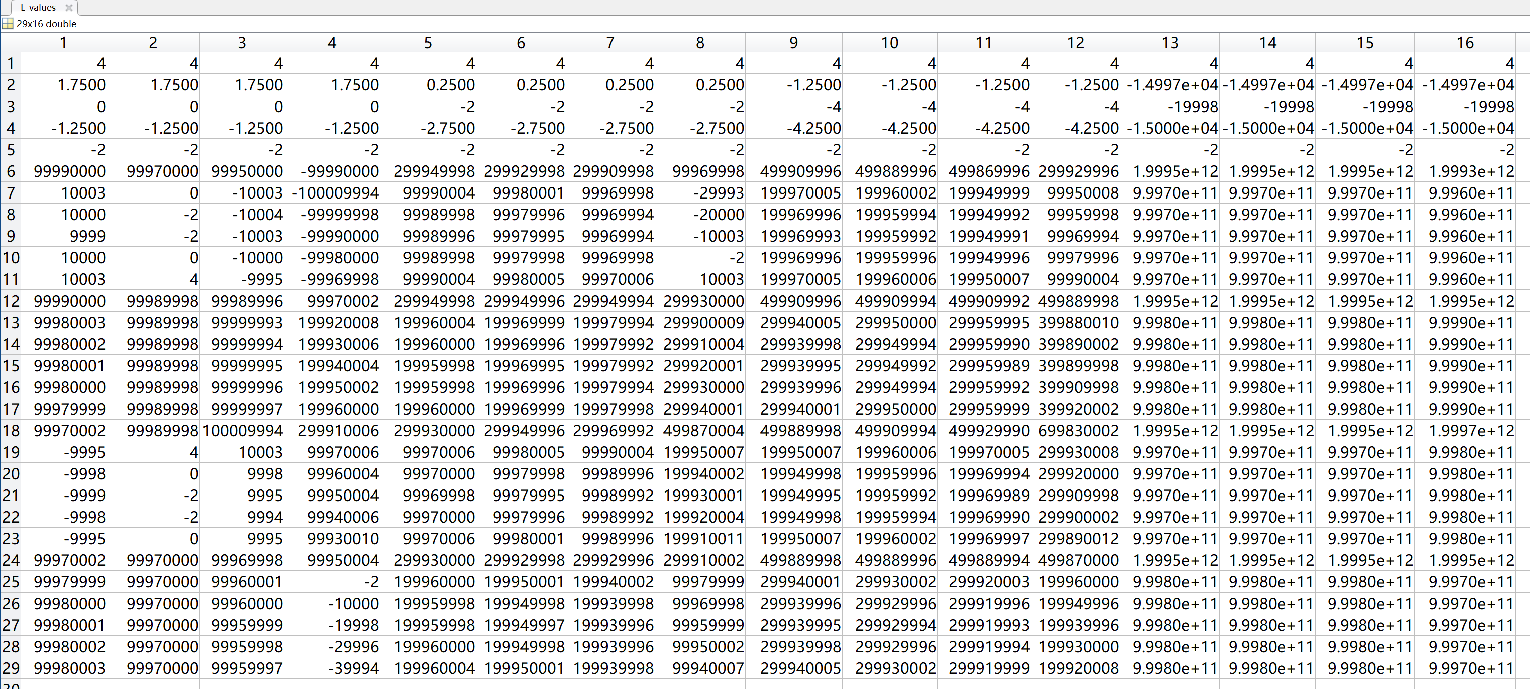
Besides, we can get \(p^*\) and \(d^*\) in this case:

1
2
3
4
5
p_star =
    -2
    
d_star =
    -2

However, although in this case we have \(d^*\le p^*\), we can’t say that the weak duality is verified, as the above matrix is only a finite part of the infinite matrix, and this \(d^*\) and \(p^*\) are probably not optimal. Having said that, this matrix can help us to better understand a Lagrange function’s primal optimization $\eqref{eq7}$ and dual optimization $\eqref{eq8}$, and the weak duality between the two.

The weak duality of general optimization problem

The above discussions about the weak duality of Lagrange function actually reflects the property of weak duality of general optimization problem $\eqref{eq11}$, and weak duality can be very useful when designing optimization problems¹:

References