Berkshire Hathaway’s Performance vs. S&P 500 and NASDAQ 100
Berkshire Hathaway’s performance vs. S&P 500
The 17th page in 2023 Berkshire Hathaway annual report1 shows a comparison between Berkshire Hathaway’s Performance and dividends included S&P 500 index from 1965 to 2023, in total 59 years. (See Appendix. BTW, it’s actually a tradition of Berkshire to compare with S&P 500 in annual reports2.) I want to visualize it using Python in this post. Here is it.
1
2
3
4
5
6
7
8
9
10
11
12
13
14
15
16
17
18
19
20
21
22
23
24
25
26
27
28
29
30
31
32
33
34
35
36
37
38
39
40
41
42
43
44
45
46
47
48
49
50
51
52
53
54
55
56
57
58
59
60
61
62
63
64
65
66
67
68
import matplotlib.pyplot as plt
from mpl_toolkits.axes_grid1 import host_subplot
%config InlineBackend.figure_format = 'svg'

years = np.array(range(1965, 2024))
num_years = np.size(years)

berkshire = np.array([49.5, -3.4, 13.3, 77.8, 19.4,
                     -4.6, 80.5, 8.1, -2.5, -48.7,
                     2.5, 129.3, 46.8, 14.5, 102.5,
                     32.8, 31.8, 38.4, 69.0, -2.7,
                     93.7, 14.2, 4.6, 59.3, 84.6,
                     -23.1, 35.6, 29.8, 38.9, 25.0,
                     57.4, 6.2, 34.9, 52.2, -19.9,
                     26.6, 6.5, -3.8, 15.8, 4.3,
                     0.8, 24.1, 28.7, -31.8, 2.7,
                     21.4, -4.7, 16.8, 32.7, 27.0,
                     -12.5, 23.4, 21.9, 2.8, 11.0,
                     2.4, 29.6, 4.0, 15.8])

sp500 = np.array([10.0, -11.7, 30.9, 11.0, -8.4,
                 3.9, 14.6, 18.9, -14.8, -26.4,
                 37.2, 23.6, -7.4, 6.4, 18.2,
                 32.3, -5.0, 21.4, 22.4, 6.1,
                 31.6, 18.6, 5.1, 16.6, 31.7,
                 -3.1, 30.5, 7.6, 10.1, 1.3,
                 37.6, 23.0, 33.4, 28.6, 21.0,
                 -9.1, -11.9, -22.1, 28.7, 10.9,
                 4.9, 15.8, 5.5, -37.0, 26.5,
                 15.1, 2.1, 16.0, 32.4, 13.7,
                 1.4, 12.0, 21.8, -4.4, 31.5,
                 18.4, 28.7, -18.1, 26.3])

idx = np.array(range(0,num_years))
years, berkshire, sp500 = years[idx], berkshire[idx], sp500[idx]

berkshire_compound, sp500_compound = np.cumprod((berkshire/100)+1), np.cumprod((sp500/100)+1)

ax1 = host_subplot(111)
ax2 = ax1.twinx()

bar_width = 0.3

ax1.bar(years, berkshire, bar_width, alpha=0.7, label='Berkshire')
ax1.bar(years+bar_width, sp500, bar_width, alpha=0.7, label='SP500')
ax1.legend(loc='upper left', ncols=2)
xticks_x, xticks_y = years+bar_width/2, years
ax1.set_xticks(xticks_x[::7], xticks_y[::7])
ax1.set_xlabel('Years')
ax1.set_ylabel('Annual percentage change (%)')

ax2.plot(years, berkshire_compound)
ax2.plot(years, sp500_compound)
ax2.set_ylabel('Overall gain')

plt.title('Berkshire''s performance vs. S&P 500 ({}-{})'.format(years[0], years[-1]))

berkshire_ag = (berkshire_compound[-1] ** (1/np.size(idx)) - 1)*100
sp500_ag = (sp500_compound[-1] ** (1/np.size(idx)) - 1)*100

print("{}-{}".format(years[0], years[-1]))
print("{}: {:.2f} ".format("Total gain (Berkshire)", berkshire_compound[-1]))
print("{}: {:.2f}%".format("Compounded annual gain (Berkshire)", berkshire_ag))
print("{}: {:.2f}".format("Total gain (SP500)", sp500_compound[-1]))
print("{}: {:.2f}%".format("Compounded annual gain (SP500)", sp500_ag))

plt.savefig("fig.png", dpi=900, bbox_inches='tight')
plt.show()
1
2
3
4
5
1965-2023
Total gain (Berkshire): 43748.51
Compounded annual gain (Berkshire): 19.86%
Total gain (SP500): 308.53
Compounded annual gain (SP500): 10.20%

We can intuitively feel the staggering power of compound rate and how great Berkshire is under Buffett’s control.
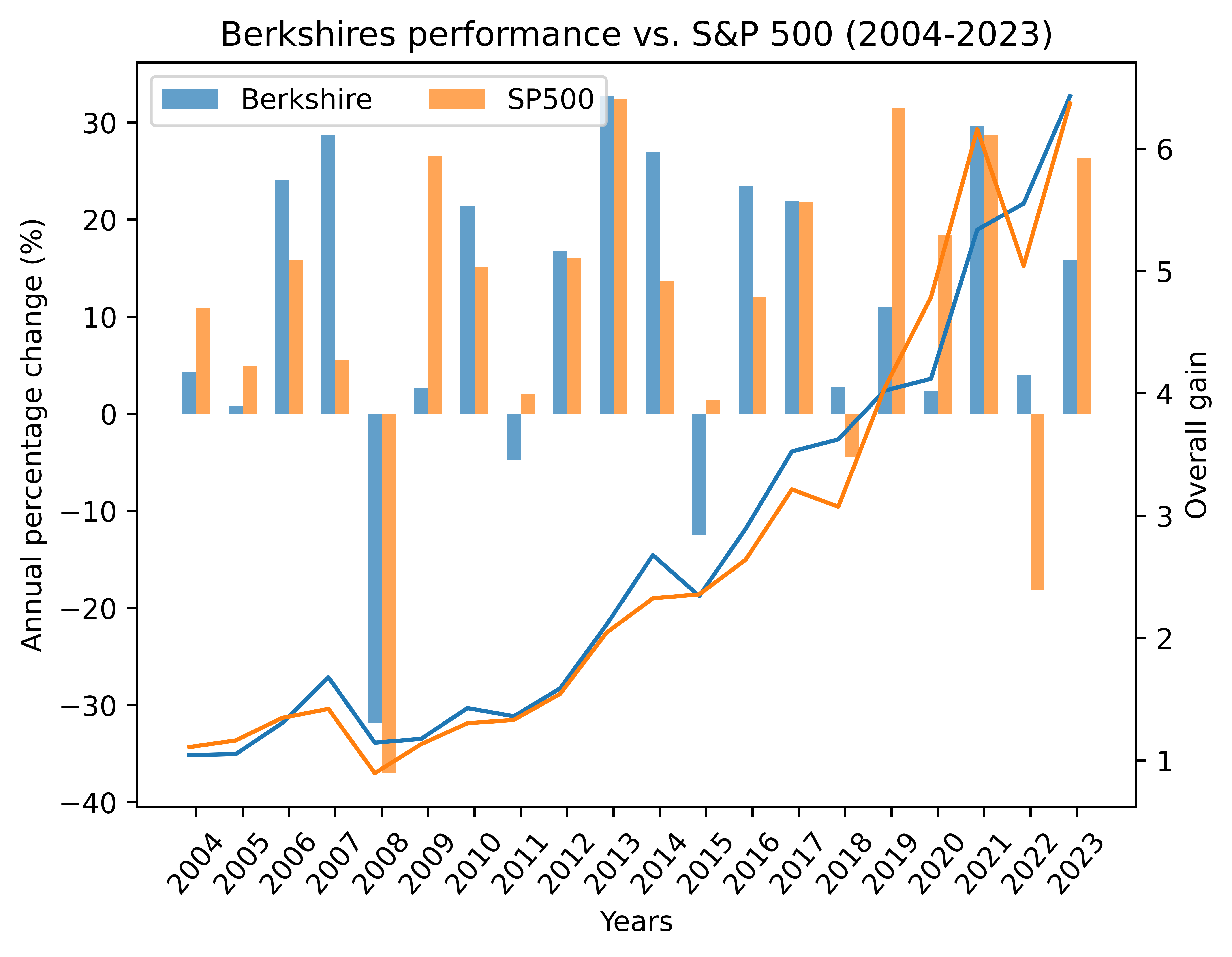
Then, we have a detailed look at performance comparison in the past 20 years:
1
2
3
4
5
6
7
8
9
10
11
# ...

idx = np.array(range(num_years-20,num_years))
years, berkshire, sp500 = years[idx], berkshire[idx], sp500[idx]

# ...

xticks_x, xticks_y = years+bar_width/2, years
ax1.set_xticks(xticks_x, xticks_y, rotation=50)

# ...
1
2
3
4
5
2004-2023
Total gain (Berkshire): 6.43
Compounded annual gain (Berkshire): 9.75%
Total gain (SP500): 6.37
Compounded annual gain (SP500): 9.70%
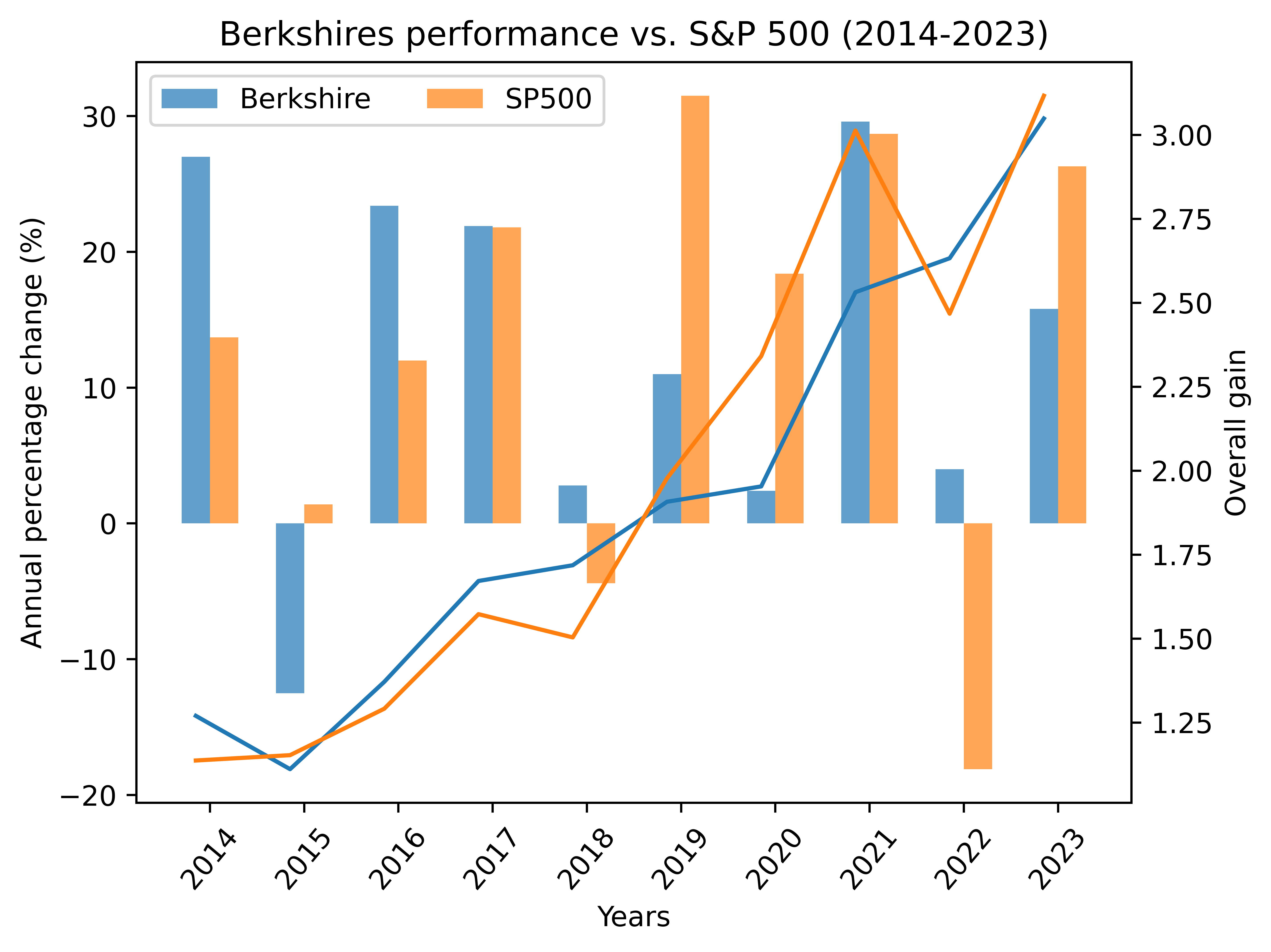
and that in the last 10 years:
1
2
3
4
5
2014-2023
Total gain (Berkshire): 3.05
Compounded annual gain (Berkshire): 11.79%
Total gain (SP500): 3.12
Compounded annual gain (SP500): 12.04%
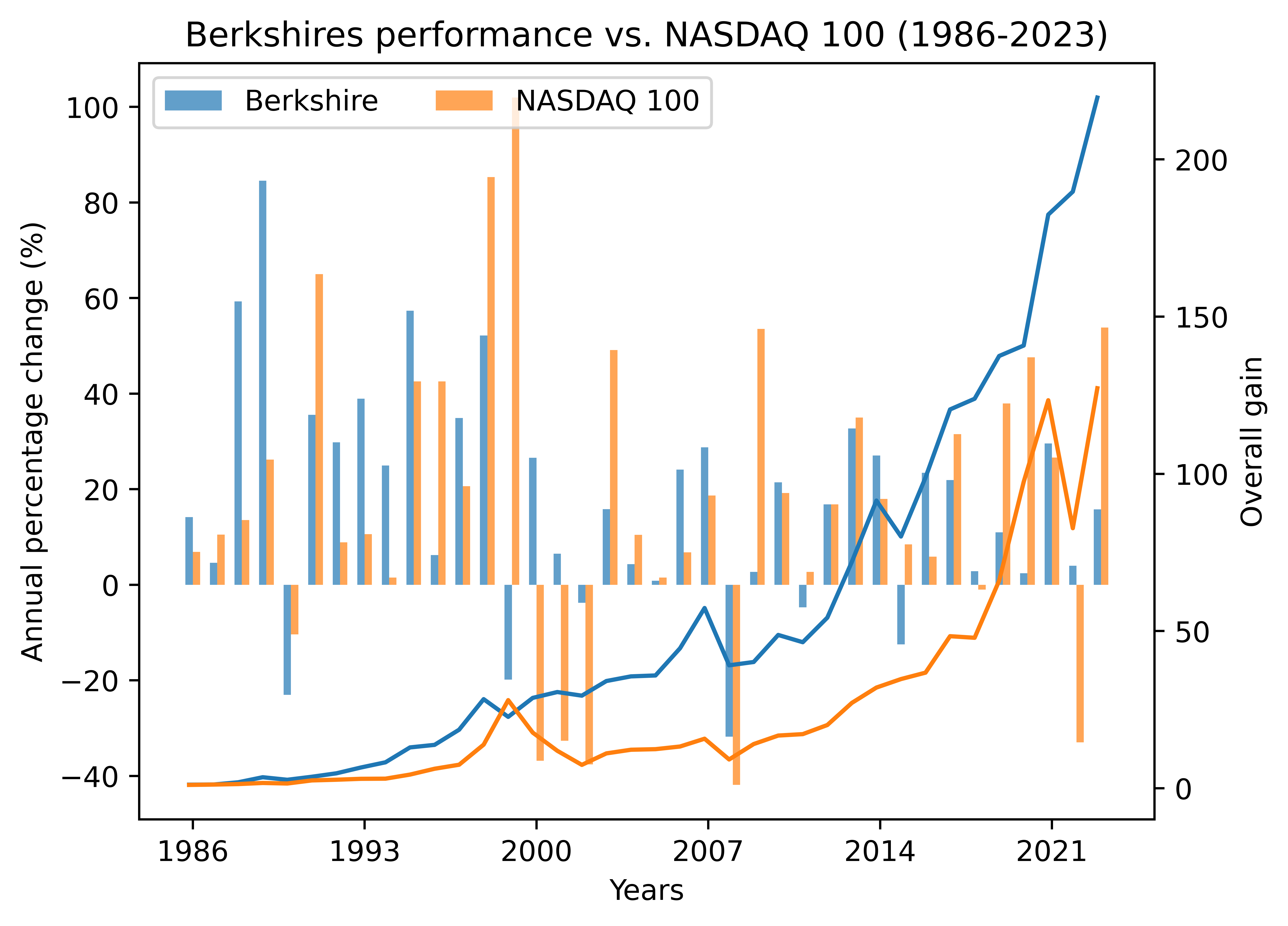
Berkshire Hathaway’s performance vs. NASDAQ 100
Yesterday (Dec. 9, 2024) , I found a website Slickcharts3, which is really close to my ideal website referenced for passive investing. It records “total returns by year” of S&P 500 (1926-2024)4, NASDAQ 100 (1986-2024)5, Dow Jones Industrial Average (1886-2024)6, and Berkshire (1981-2024)7.
In the following text, I would compare Berkshire’s performance with NASDAQ 100 as I did as above. By the way, at this time the Berkshire’s annual returns I adopt are from website Slickcharts7, rather than official annual report.
1
2
3
4
5
6
7
8
9
10
11
12
13
14
15
16
17
18
19
20
21
22
23
24
25
26
27
28
29
30
31
32
33
34
35
36
37
38
39
40
41
42
43
44
45
46
47
48
49
50
51
52
53
54
55
56
57
58
59
60
import matplotlib.pyplot as plt
from mpl_toolkits.axes_grid1 import host_subplot
%config InlineBackend.figure_format = 'svg'

years = np.array(range(1986, 2024))
num_years = np.size(years)

berkshire = np.array([14.17, 4.61, 59.32, 84.57, -23.05,
                     35.58, 29.83, 38.94, 24.96, 57.35,
                     6.23, 34.90, 52.17, -19.86, 26.56,
                     6.48, -3.77, 15.81, 4.33, 0.82,
                     24.11, 28.74, -31.78, 2.69, 21.42,
                     -4.73, 16.82, 32.70, 27.04, -12.48,
                     23.42, 21.91, 2.82, 10.98, 2.42,
                     29.57, 4.00, 15.77])

nasaq100 = np.array([6.89, 10.50, 13.54, 26.17, -10.41,
                    64.99, 8.86, 10.58, 1.50, 42.54,
                    42.54, 20.63, 85.30, 101.95, -36.84,
                    -32.65, -37.58, 49.12, 10.44, 1.49,
                    6.79, 18.67, -41.89, 53.54, 19.22,
                    2.70, 16.82, 34.99, 17.94, 8.43,
                    5.89, 31.52, -1.04, 37.96, 47.58,
                    26.63, -32.97, 53.81])

idx = np.array(range(0,num_years))
years, berkshire, nasaq100 = years[idx], berkshire[idx], nasaq100[idx]

berkshire_compound, sp500_compound = np.cumprod((berkshire/100)+1), np.cumprod((nasaq100/100)+1)

ax1 = host_subplot(111)
ax2 = ax1.twinx()

bar_width = 0.3

ax1.bar(years, berkshire, bar_width, alpha=0.7, label='Berkshire')
ax1.bar(years+bar_width, nasaq100, bar_width, alpha=0.7, label='NASDAQ 100')
ax1.legend(loc='upper left', ncols=2)
xticks_x, xticks_y = years+bar_width/2, years
ax1.set_xticks(xticks_x[::7], xticks_y[::7])
ax1.set_xlabel('Years')
ax1.set_ylabel('Annual percentage change (%)')

ax2.plot(years, berkshire_compound)
ax2.plot(years, sp500_compound)
ax2.set_ylabel('Overall gain')

plt.title('Berkshire''s performance vs. NASDAQ 100 ({}-{})'.format(years[0], years[-1]))

berkshire_ag = (berkshire_compound[-1] ** (1/np.size(idx)) - 1)*100
sp500_ag = (sp500_compound[-1] ** (1/np.size(idx)) - 1)*100

print("{}-{}".format(years[0], years[-1]))
print("{}: {:.2f} ".format("Total gain (Berkshire)", berkshire_compound[-1]))
print("{}: {:.2f}%".format("Compounded annual gain (Berkshire)", berkshire_ag))
print("{}: {:.2f}".format("Total gain (NASDAQ 100)", sp500_compound[-1]))
print("{}: {:.2f}%".format("Compounded annual gain (NASDAQ 100)", sp500_ag))

plt.savefig("fig.png", dpi=900, bbox_inches='tight')
plt.show()
1
2
3
4
5
1986-2023
Total gain (Berkshire): 219.65
Compounded annual gain (Berkshire): 15.25%
Total gain (NASDAQ 100): 127.22
Compounded annual gain (NASDAQ 100): 13.60%
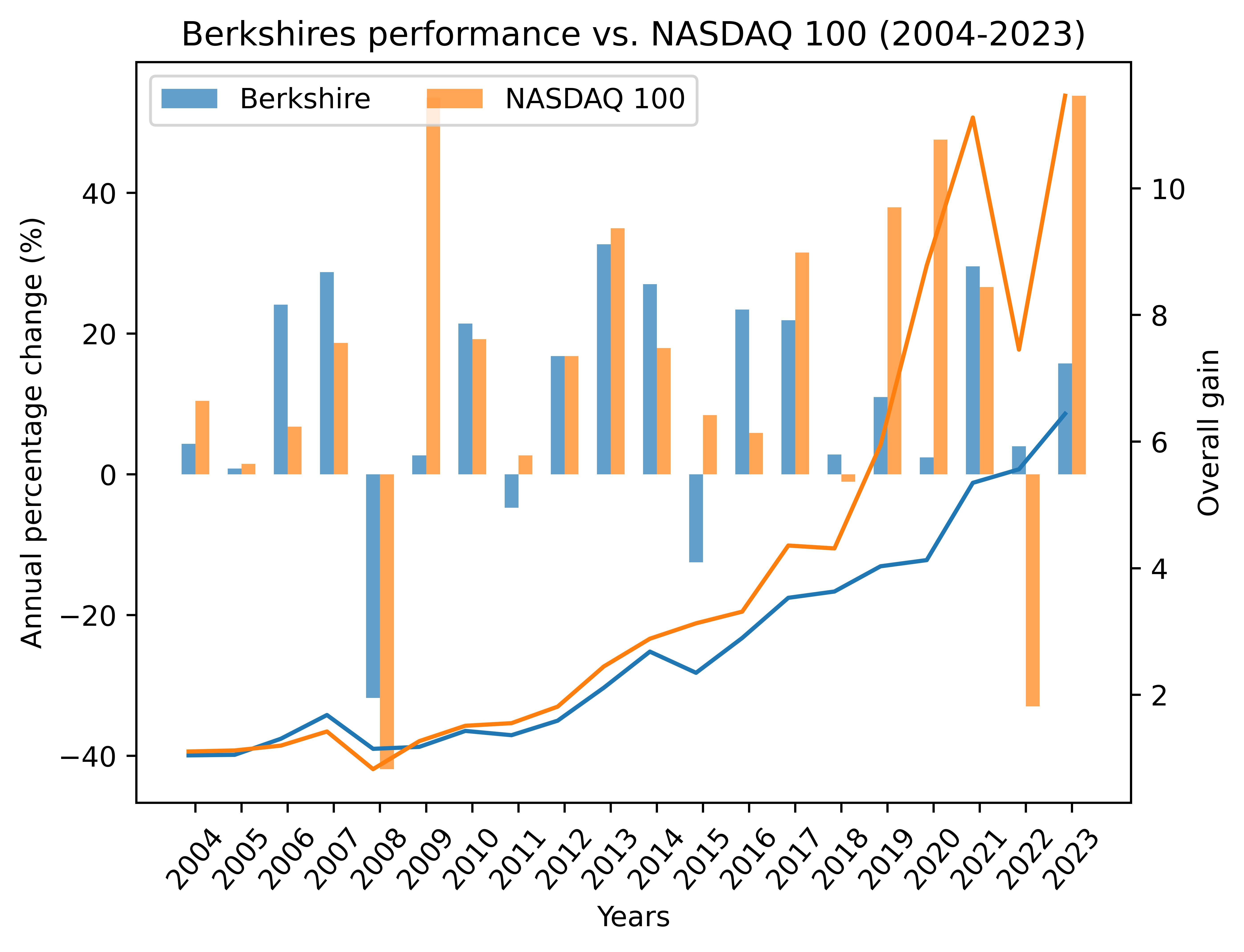
Similarly, we can have a comparison of the last 20 years:
1
2
3
4
5
6
7
8
9
10
11
# ...

idx = np.array(range(num_years-20,num_years))
years, berkshire, nasaq100 = years[idx], berkshire[idx], nasaq100[idx]

# ...

xticks_x, xticks_y = years+bar_width/2, years
ax1.set_xticks(xticks_x, xticks_y, rotation=50)

# ...
1
2
3
4
5
2004-2023
Total gain (Berkshire): 6.44
Compounded annual gain (Berkshire): 9.76%
Total gain (NASDAQ 100): 11.46
Compounded annual gain (NASDAQ 100): 12.97%
and the last 10 years:
1
2
3
4
5
2014-2023
Total gain (Berkshire): 3.05
Compounded annual gain (Berkshire): 11.80%
Total gain (NASDAQ 100): 4.68
Compounded annual gain (NASDAQ 100): 16.70%
The power of each compound interest
At last, take compounded annual gain of Berkshire and S&P 500 (19.86% and 10.20% respectively) and NASDAQ 100 (13.60%), we can calculate how \$1 compounds every 5 years with each compound interest.
1
2
3
4
5
6
7
8
9
10
11
12
13
import numpy as np
from pandas import DataFrame

years = np.array(range(5,65,5))
berkshire, sp500, nasdaq100 = (1+0.1986) ** years, (1+0.1020) ** years, (1+0.1360) ** years

data = DataFrame({'Years': years,
       'Berkshire': berkshire,
       'S&P 500': sp500,
       'NASDAQ 100': nasdaq100})
data = data.set_index('Years')

print(data)
1
2
3
4
5
6
7
8
9
10
11
12
13
14
          Berkshire     S&P 500   NASDAQ 100
Years
5          2.473839    1.625204     1.891872
10         6.119878    2.641289     3.579178
15        15.139590    4.292635     6.771345
20        37.452901    6.976408    12.810516
25        92.652434   11.338089    24.235852
30       229.207171   18.426711    45.851119
35       567.021554   29.947171    86.744430
40      1402.719823   48.670273   164.109323
45      3470.102484   79.099138   310.473768
50      8584.473573  128.552263   587.376502
55     21236.602338  208.923695  1111.240921
60     52535.927219  339.543695  2102.325134
Note: In the annual report, the time period adopted when calculating “Compound Annual Gain” and “Overall Gain” is sort of different, reflected in that the former starts from 1965 while the latter 1964. This point should be noted when comparing them with my calculation results.
References