Fetch Series Data from FRED Sever in Python: take S&P 500 price index

Aug. 05, 2024

Python `pyfredapi`

I ever tried to fetch series data from FRED (Federal Reserve Economic Data) server using MATLAB¹, and in this post, I’m going to learn how to do so with the help of pyfredapi²³ package in Python.

First, install pyfredapi by:

pip install pyfredapi

Different from MATLAB fred function, an API key must be specified when fetching data from FRED server² by pyfredapi functions. So, we should register an account⁴ at first and then apply for an API key.

Next, as for how to use API key, pyfredapi package provides two ways²:

You can set your API key in two ways:

set your API key to the environment variable FRED_API_KEY (specify in ~/.zshrc, ~/.bashrc file)
pass it to the api_key parameter of the request function

For the first one, files zshrc and bashrc seem not compatible with Windows systems. So, as will be shown below, I adopt the second way. And, for the sake of confidentiality, I will use <my_api_key> to implicitly represent my own API key.

Then, let’s take S&P 500 price index to look at those fundamental pyfredapi functions³.

`pyfredapi.series.get_series_info` function

At first, the package provides pyfredapi.series.get_series_info function⁵ to obtain series information:

You can query a series’ information directly with get_series_info. The get_series_info function returns a SeriesInfo object that contains all the metadata for the given series.²

For example:

import pyfredapi as pf
from rich import print as rprint
from rich.pretty import pprint

SP500_info = pf.get_series_info(series_id="SP500", api_key="<my_api_key>")

# Using rich to pretty print the SeriesInfo
rprint(SP500_info)

SeriesInfo(
    id='SP500',
    realtime_start='2024-08-04',
    realtime_end='2024-08-04',
    title='S&P 500',
    observation_start='2014-08-04',
    observation_end='2024-08-02',
    frequency='Daily, Close',
    frequency_short='D',
    units='Index',
    units_short='Index',
    seasonal_adjustment='Not Seasonally Adjusted',
    seasonal_adjustment_short='NSA',
    last_updated='2024-08-02 19:57:09-05',
    popularity=83,
    notes='The observations for the S&P 500 represent the daily index value at market close. The market typically 
closes at 4 PM ET, except for holidays when it sometimes closes early.\r\n\r\nThe Federal Reserve Bank of St. Louis
and S&P Dow Jones Indices LLC have reached a new agreement on the use of Standard & Poors and Dow Jones Averages 
series in FRED. FRED and its associated services will include 10 years of daily history for Standard & Poors and 
Dow Jones Averages series.\r\n\r\nThe S&P 500 is regarded as a gauge of the large cap U.S. equities market. The 
index includes 500 leading companies in leading industries of the U.S. economy, which are publicly held on either 
the NYSE or NASDAQ, and covers 75% of U.S. equities. Since this is a price index and not a total return index, the 
S&P 500 index here does not contain dividends.\r\n\r\nCopyright © 2016, S&P Dow Jones Indices LLC. All rights 
reserved. Reproduction of S&P 500 in any form is prohibited except with the prior written permission of S&P Dow 
Jones Indices LLC ("S&P"). S&P does not guarantee the accuracy, adequacy, completeness or availability of any 
information and is not responsible for any errors or omissions, regardless of the cause or for the results obtained
from the use of such information. S&P DISCLAIMS ANY AND ALL EXPRESS OR IMPLIED WARRANTIES, INCLUDING, BUT NOT 
LIMITED TO, ANY WARRANTIES OF MERCHANTABILITY OR FITNESS FOR A PARTICULAR PURPOSE OR USE. In no event shall S&P be 
liable for any direct, indirect, special or consequential damages, costs, expenses, legal fees, or losses 
(including lost income or lost profit and opportunity costs) in connection with subscriber\'s or others\' use of 
S&P 500.\r\n\r\nPermission to reproduce S&P 500 can be requested from index_services@spdji.com. More contact 
details are available here (http://us.spindices.com/contact-us), including phone numbers for all regional offices.'
)

SP500_info is a pyfredapi.series.SeriesInfo type object:

type(SP500_info)

pyfredapi.series.SeriesInfo

and we can use . operator to get value of particular attribute, for example:

print("id:", SP500_info.id, "\nfrequency:", SP500_info.frequency)

id: SP500 
frequency: Daily, Close

Here are all available attributes and methods of pyfredapi.series.SeriesInfo object:

dir(SP500_info)

['Config',
 '__abstractmethods__',
 '__annotations__',
 '__class__',
 '__class_vars__',
 '__config__',
 '__custom_root_type__',
 '__delattr__',
 '__dict__',
 '__dir__',
 '__doc__',
 '__eq__',
 '__exclude_fields__',
 '__fields__',
 '__fields_set__',
 '__format__',
 '__ge__',
 '__get_validators__',
 '__getattribute__',
 '__getstate__',
 '__gt__',
 '__hash__',
 '__include_fields__',
 '__init__',
 '__init_subclass__',
 '__iter__',
 '__json_encoder__',
 '__le__',
 '__lt__',
 '__module__',
 '__ne__',
 '__new__',
 '__post_root_validators__',
 '__pre_root_validators__',
 '__pretty__',
 '__private_attributes__',
 '__reduce__',
 '__reduce_ex__',
 '__repr__',
 '__repr_args__',
 '__repr_name__',
 '__repr_str__',
 '__rich_repr__',
 '__schema_cache__',
 '__setattr__',
 '__setstate__',
 '__signature__',
 '__sizeof__',
 '__slots__',
 '__str__',
 '__subclasshook__',
 '__try_update_forward_refs__',
 '__validators__',
 '_abc_impl',
 '_base_url',
 '_calculate_keys',
 '_copy_and_set_values',
 '_decompose_class',
 '_enforce_dict_if_root',
 '_get_value',
 '_init_private_attributes',
 '_iter',
 'construct',
 'copy',
 'dict',
 'frequency',
 'frequency_short',
 'from_orm',
 'id',
 'json',
 'last_updated',
 'notes',
 'observation_end',
 'observation_start',
 'open_url',
 'parse_file',
 'parse_obj',
 'parse_raw',
 'popularity',
 'realtime_end',
 'realtime_start',
 'schema',
 'schema_json',
 'seasonal_adjustment',
 'seasonal_adjustment_short',
 'title',
 'units',
 'units_short',
 'update_forward_refs',
 'validate']

As shown before, pyfredapi.series.SeriesInfo objects provide an open_url method⁶ to “open the FRED webpage for the given series”. In this case, running SP500_info.open_url() will make browser open and jump to webpage https://fred.stlouisfed.org/series/SP500.

At the beginning, I didn’t know I should have provided an API key—I just use gdp_info = pf.get_series_info(series_id="GDP") in the script, with no API key, so I had an error:

---------------------------------------------------------------------------
APIKeyNotFound                            Traceback (most recent call last)
Cell In[8], line 5
      2 from rich import print as rprint
      3 from rich.pretty import pprint
----> 5 gdp_info = pf.get_series_info(series_id="GDP")
      7 # Using rich to pretty print the SeriesInfo
      8 rprint(gdp_info)

...

APIKeyNotFound: API key not found. Either set a FRED_API_KEY environment variable or pass your API key to the `api_key` parameter.

Look out this point.

The script is basically the same as the official example in³, and in which a Python package rich is imported. It is to display “rich text and beautiful formatting in the terminal.”⁷ In this case, rich.print makes print information more readable and colorful (at least in Jupyter Notebook).

`pyfredapi.series.get_series` function

pyfredapi.get_series_info is to obtain particular series information via API, and pyfredapi.series.get_series⁸ is to fetch corresponding series data:

Parameters

series_id: Series id of interest.
api_key=None: FRED API key. Defaults to None. If None, will search for FRED_API_KEY in environment variables.
return_format='pandas': Define how to return the response. Must be either ‘json’ or ‘pandas’. Defaults to ‘pandas’.
kwargs: dict, (optional): Additional parameters to FRED API series/observations endpoint. Refer to the FRED documentation for a list of all possible parameters.

Returns

Either a dictionary representing the json response or a pandas dataframe.

Return type

dict | pd.DataFrame

For example:

SP500_df = pf.get_series(series_id="SP500", api_key="<my_api_key>")
SP500_df.tail()

	realtime_start	realtime_end	date	value
2605	2024-08-02	2024-08-02	2024-07-29	5463.54
2606	2024-08-02	2024-08-02	2024-07-30	5436.44
2607	2024-08-02	2024-08-02	2024-07-31	5522.30
2608	2024-08-02	2024-08-02	2024-08-01	5446.68
2609	2024-08-02	2024-08-02	2024-08-02	5346.56

where SP500_df is a Pandas DataFrame object:

type(SP500_df)

pandas.core.frame.DataFrame

and data type of each column is:

SP500_df.dtypes

realtime_start            object
realtime_end              object
date              datetime64[ns]
value                    float64
dtype: object

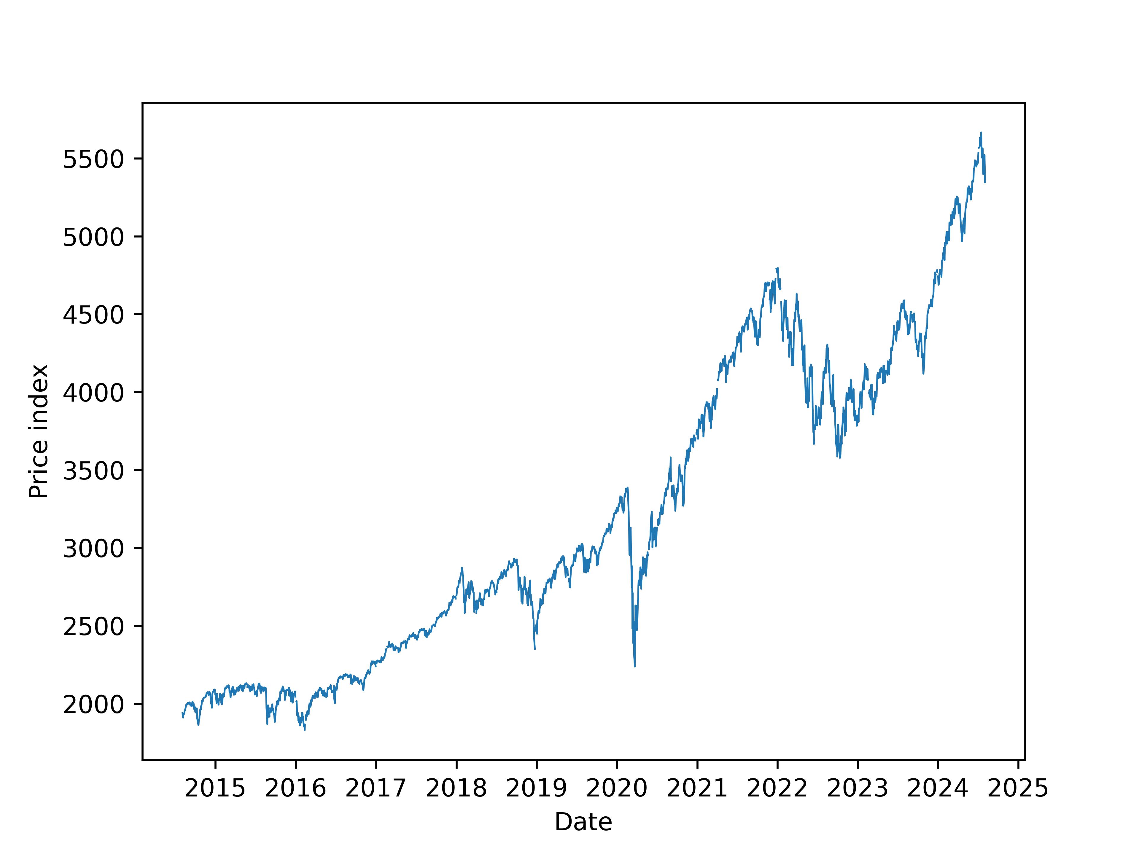
We can visualize how S&P 500 price index changes as date:

import matplotlib.pyplot as plt
%config InlineBackend.figure_format = 'svg'

plt.plot(SP500_df['date'], SP500_df['value'], linewidth=0.7)
plt.xlabel('Date')
plt.ylabel('Price index')
plt.savefig("fig-1.jpg", dpi=600)

fig-1

As in the introduction to get_series, besides Pandas DataFrame, we can also choose to return series data in JSON format, that is:

sp500_json = pf.get_series(series_id="SP500", api_key="<my_api_key>", return_format='json')
pprint(sp500_json, max_length=5)

[
│   {'realtime_start': '2024-08-02', 'realtime_end': '2024-08-02', 'date': '2014-08-04', 'value': '1938.99'},
│   {'realtime_start': '2024-08-02', 'realtime_end': '2024-08-02', 'date': '2014-08-05', 'value': '1920.21'},
│   {'realtime_start': '2024-08-02', 'realtime_end': '2024-08-02', 'date': '2014-08-06', 'value': '1920.24'},
│   {'realtime_start': '2024-08-02', 'realtime_end': '2024-08-02', 'date': '2014-08-07', 'value': '1909.57'},
│   {'realtime_start': '2024-08-02', 'realtime_end': '2024-08-02', 'date': '2014-08-08', 'value': '1931.59'},
│   ... +2605
]

In addition, we can specify series time range (if available), for example:

SP500_df = pf.get_series(series_id="SP500", api_key="<my_api_key>", 
                        observation_start='2017-10-17', observation_end='2019-10-17')
plt.plot(SP500_df['date'], SP500_df['value'], linewidth=0.7)
plt.xlabel('Date')
plt.ylabel('Price index')
plt.xticks(rotation=45)
plt.savefig("fig-2.jpg", dpi=600, bbox_inches='tight')

fig-2

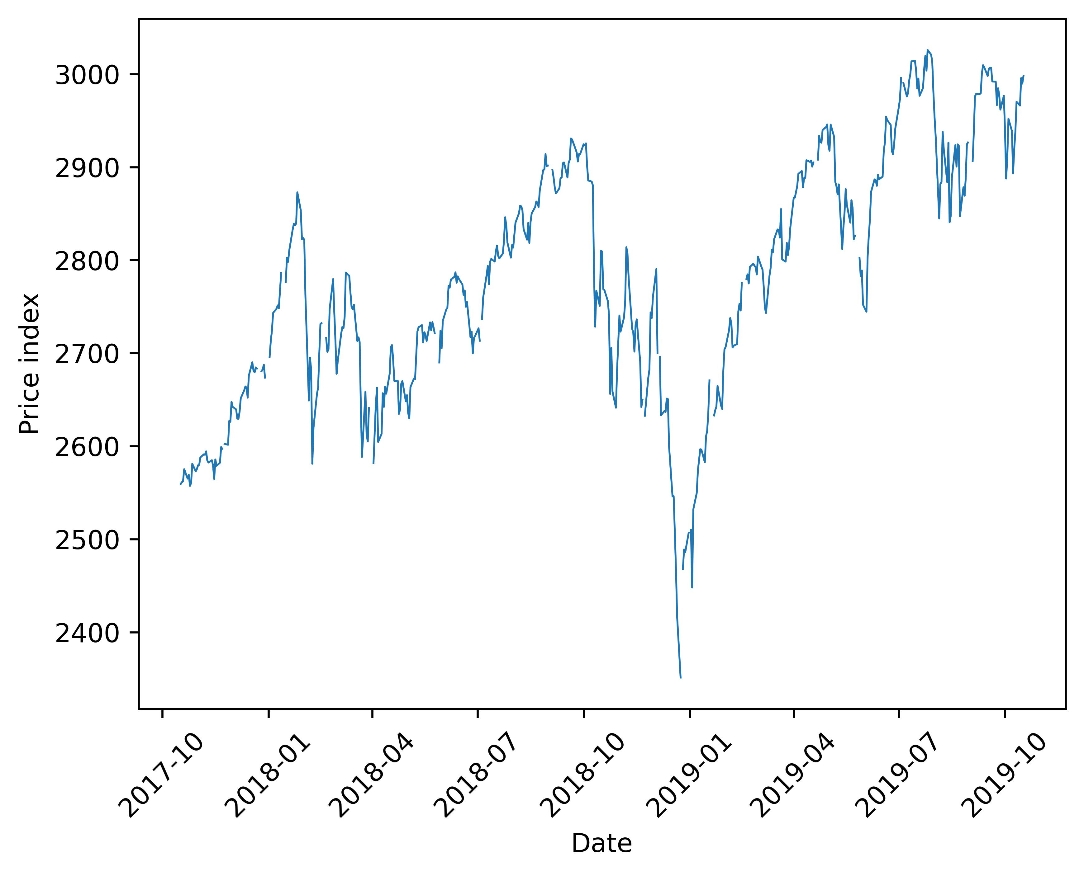
In this case, observation_start and observation_end are “Additional parameters to FRED API series/observations endpoint” as said in the introduction. Besides the two, more parameters can be found in FRED documentation⁹. In addition, FRED API documentation¹⁰ is really informative.

Archival series data: ALFRED

No matter in blog¹ or in above practice, the series I fetch is FRED data. During the learning process, I found another kind of series provided, i.e. ALFRED, which is the archived version of FRED:

ALFRED®¹¹

ALFRED® stands for Archival Federal Reserve Economic Data. ALFRED® archives FRED® data by adding the real-time period when values were originally released and later revised. For instance on February 2, 1990, the US Bureau of Labor Statistics reported the US unemployment rate for the month of January, 1990 as 5.3 percent. Over 6 years later on March 8, 1996, the US unemployment rate for the same month January, 1990 was revised to 5.4 percent.

FRED® versus ALFRED®¹²

Most users are interested in FRED® and not ALFRED®. In other words, most people want to know what’s the most accurate information about the past that is available today (FRED®) not what information was known on some past date in history (ALFRED®).

Note that the FRED® and ALFRED® web services use the same URLs but with different options. The default options for each URL have been chosen to make the most sense for FRED® users. In particular by default, the real-time period has been set to today’s date. ALFRED® users can change the real-time period by setting the realtime_start and realtime_end variables.

Very rigorous.

Certainly, package pyfredapi also supports accessing ALFRED data, and I’ll get into it in the future if necessary.

References

Python pyfredapi

pyfredapi.series.get_series_info function

pyfredapi.series.get_series function

Archival series data: ALFRED

Python `pyfredapi`

`pyfredapi.series.get_series_info` function

`pyfredapi.series.get_series` function