A Simple Example to Know about CycleGAN

Jul. 27, 2024

The book, Deep Learning with PyTorch (Subchapter 2.2, A pretrained model that fakes it until it makes it), simply introduces CycleGAN and provides a practice about it¹:

… A CycleGAN can return images of one domain into images of another domain (and back), without the need for us to explicitly provide matching pairs in the training set.

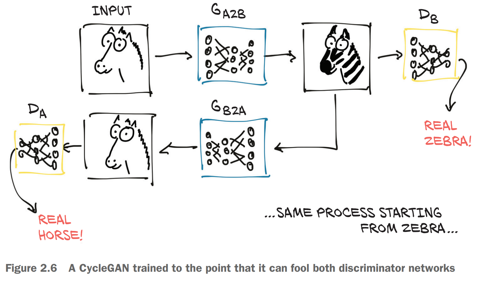
In figure 2.6, we have a CycleGAN workflow for the task of turning a photo of a horse into a zebra, and vice versa. Note that there are two separate generator networks, as well as two distinct discriminators.

As the figure shows, the first generator learns to produce an image conforming to a target distribution (zebras, in this case) starting from an image belonging to a different distribution (horses), so that the discriminator can’t tell if the image produced from a horse photo is actually a genuine picture of a zebra or not. At the same time—and here’s where the Cycle prefix in the acronym comes in—the resulting fake zebra is sent through a different generator going the other way (zebra to horse, in our case), to be judged by another discriminator on the other side. Creating such a cycle stabilizes the training process considerably, which addresses one of the original issues with GANs.

The fun part is that at this point, we don’t need matched horse/zebra pairs as ground truths (good luck getting them to match poses!). It’s enough to start from a collection of unrelated horse images and zebra photos for the generators to learn their task, going beyond a purely supervised setting. The implications of this model go even further than this: the generator learns how to selectively change the appearance of objects in the scene without supervision about what’s what. There’s no signal indicating that manes are manes and legs are legs, but they get translated to something that lines up with the anatomy of the other animal.

I ever heard about CycleGAN, but didn’t get into it before, just thinking that “cycle” indicates a novel network structure, like making several networks forming a circle or whatever. Now, I realize it’s more about function — realize bidirectional conversion between two domain images (or other information). Another point is that, the training mode of CycleGAN is unsupervised, which means that we don’t need to undertake laborious labeling task when preparing dataset.

Next, the book takes a specify CycleGAN to show how to use it (actually part of it, i.e. $\text{G}_{\text{A2B}}$ in above figure):

… The CycleGAN network [as will be showed below] has been trained on a dataset of (unrelated) horse images and zebra images extracted from the ImageNet dataset. The network learns to take an image of one or more horses and turn them all into zebras, leaving the rest of the image as unmodified as possible. While humankind hasn’t held its breath over the last few thousand years for a tool that turn horses into zebras, this task showcases the ability of these architectures to model complex real-world processes with distant supervision [more information about distant supervision can refer to²].

… that we would run a generator model that had been pretrained on the horse2zebra dataset, whose training set contains two sets of 1068 and 1335 images of horses and zebras, respectively.

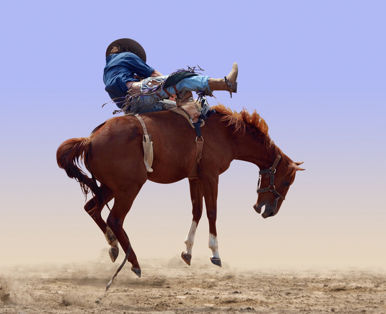
Specifically, its function is to convert image like horse.jpg:

horse

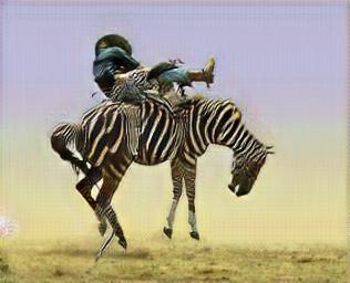
to zebra.jpg:

zebra

and complete code shows as follows:

import torch

# Instantiate the class `ResNetGenerator` with a set of pretrained parameters
netG = ResNetGenerator()
model_path = 'horse2zebra_0.4.0.pth'
model_data = torch.load(model_path)
netG.load_state_dict(model_data)

# Put the model in eval mode
netG.eval()

from PIL import Image
from torchvision import transforms

# Load an image and preprocess it
img = Image.open('horse.jpg') # img.size: (1500, 1220)
preprocess = transforms.Compose([transforms.Resize(256),
                                transforms.ToTensor()])
img_t = preprocess(img) # img_t.size(): torch.Size([3, 256, 314])
batch_t = torch.unsqueeze(img_t, 0) # batch_t.size(): torch.Size([1, 3, 256, 314])

# Send the preprocessed image to Generator
batch_out = netG(batch_t) # batch_out.size(): torch.Size([1, 3, 256, 316])

# Convert back to an image
out_t = (batch_out.data.squeeze() + 1.0) / 2.0 # batch_out.data.squeeze().size(): torch.Size([3, 256, 316])
out_img = transforms.ToPILImage()(out_t)
out_img.save('zebra.jpg')

Required files

horse2zebra_0.4.0.pth: https://github.com/deep-learning-with-pytorch/dlwpt-code/blob/master/data/p1ch2/horse2zebra_0.4.0.pth.
horse.jpg: https://github.com/deep-learning-with-pytorch/dlwpt-code/blob/master/data/p1ch2/horse.jpg.

Notes

(1) This code snippet only shows how to use a pretrained generator of CycleGAN, without illustrating more information about another generator, that is $\text{G}_{\text{B2A}}$ in the figure, and those two discriminators, $\text{D}_{\text{B}}$ and $\text{D}_{\text{A}}$, and the whole training process (the book intentionally arranged in this way, “… the implementation isn’t relevant right now, and it’s too complex to follow until we’ve gotten a lot more PyTorch experience. Right now, we’re focused on what it can do, rather than how it does it.”). Anyway, it’s still an example of model inference³.

(2) The definition of ResNetGenerator class can be found in the appendix, and its basic component is ResNet bottleneck³.

(3) Note the way of loading a set of pretrained weights in this example. .pth pickle file is usually used for storing PyTorch state dictionary, that is the state of a PyTorch model, including weights, biases and other parameters⁴, and we can use torch.load function to load it⁵⁶. For this case, we can simply verify this point by just printing dictionary key values:

for key in model_data.keys():
    print(key)

model.1.weight
model.1.bias
model.4.weight
model.4.bias
model.7.weight
model.7.bias
model.10.conv_block.1.weight
model.10.conv_block.1.bias
model.10.conv_block.5.weight
model.10.conv_block.5.bias
model.11.conv_block.1.weight
model.11.conv_block.1.bias
model.11.conv_block.5.weight
model.11.conv_block.5.bias
model.12.conv_block.1.weight
model.12.conv_block.1.bias
model.12.conv_block.5.weight
model.12.conv_block.5.bias
model.13.conv_block.1.weight
model.13.conv_block.1.bias
model.13.conv_block.5.weight
model.13.conv_block.5.bias
model.14.conv_block.1.weight
model.14.conv_block.1.bias
model.14.conv_block.5.weight
model.14.conv_block.5.bias
model.15.conv_block.1.weight
model.15.conv_block.1.bias
model.15.conv_block.5.weight
model.15.conv_block.5.bias
model.16.conv_block.1.weight
model.16.conv_block.1.bias
model.16.conv_block.5.weight
model.16.conv_block.5.bias
model.17.conv_block.1.weight
model.17.conv_block.1.bias
model.17.conv_block.5.weight
model.17.conv_block.5.bias
model.18.conv_block.1.weight
model.18.conv_block.1.bias
model.18.conv_block.5.weight
model.18.conv_block.5.bias
model.19.weight
model.19.bias
model.22.weight
model.22.bias
model.26.weight
model.26.bias

To my understandings, it is a “lightweight” method to save and load model by .pth file, because this kind of file only stores parameters, not including model structure, and I think which is why we have to declare ResNetBlock class even if we just want to make a model inference. I guess there should be some methods to save complete model instead.

Appendix

ResNetGenerator class:

import torch
import torch.nn as nn

class ResNetBlock(nn.Module):

    def __init__(self, dim):
        super(ResNetBlock, self).__init__()
        self.conv_block = self.build_conv_block(dim)

    def build_conv_block(self, dim):
        conv_block = []

        conv_block += [nn.ReflectionPad2d(1)]

        conv_block += [nn.Conv2d(dim, dim, kernel_size=3, padding=0, bias=True),
                       nn.InstanceNorm2d(dim),
                       nn.ReLU(True)]

        conv_block += [nn.ReflectionPad2d(1)]

        conv_block += [nn.Conv2d(dim, dim, kernel_size=3, padding=0, bias=True),
                       nn.InstanceNorm2d(dim)]

        return nn.Sequential(*conv_block)

    def forward(self, x):
        out = x + self.conv_block(x) # <2>
        return out


class ResNetGenerator(nn.Module):

    def __init__(self, input_nc=3, output_nc=3, ngf=64, n_blocks=9): # <3> 

        assert(n_blocks >= 0)
        super(ResNetGenerator, self).__init__()

        self.input_nc = input_nc
        self.output_nc = output_nc
        self.ngf = ngf

        model = [nn.ReflectionPad2d(3),
                 nn.Conv2d(input_nc, ngf, kernel_size=7, padding=0, bias=True),
                 nn.InstanceNorm2d(ngf),
                 nn.ReLU(True)]

        n_downsampling = 2
        for i in range(n_downsampling):
            mult = 2**i
            model += [nn.Conv2d(ngf * mult, ngf * mult * 2, kernel_size=3,
                                stride=2, padding=1, bias=True),
                      nn.InstanceNorm2d(ngf * mult * 2),
                      nn.ReLU(True)]

        mult = 2**n_downsampling
        for i in range(n_blocks):
            model += [ResNetBlock(ngf * mult)]

        for i in range(n_downsampling):
            mult = 2**(n_downsampling - i)
            model += [nn.ConvTranspose2d(ngf * mult, int(ngf * mult / 2),
                                         kernel_size=3, stride=2,
                                         padding=1, output_padding=1,
                                         bias=True),
                      nn.InstanceNorm2d(int(ngf * mult / 2)),
                      nn.ReLU(True)]

        model += [nn.ReflectionPad2d(3)]
        model += [nn.Conv2d(ngf, output_nc, kernel_size=7, padding=0)]
        model += [nn.Tanh()]

        self.model = nn.Sequential(*model)

    def forward(self, input):
        return self.model(input)

We can instantiate it and use netron package to visualize whose network structure⁷:

import netron
import torch.onnx

netG = ResNetGenerator()
model_path = 'horse2zebra_0.4.0.pth'
model_data = torch.load(model_path)
netG.load_state_dict(model_data)
netG.eval()

x = torch.randn(1, 3, 256, 314)
modelFile = "netG.pth"
torch.onnx.export(netG, x, modelFile)
netron.start(modelFile)

netG.pth

References

Deep Learning with PyTorch, Eli Stevens, Luca Antiga, and Thomas Viehmann, 2020, GitHub repository: deep-learning-with-pytorch, pp. 27-33. ˄
… An alternative approach to generating training data is distant supervision. In distant supervision, we make use of an already existing database, such as Freebase or a domain-specific database, to collect examples for the relation we want to extract. We then use these examples to automatically generate our training data. For example, Freebase contains the fact that Barack Obama and Michelle Obama are married. We take this fact, and then label each pair of “Barack Obama” and “Michelle Obama” that appear in the same sentence as a positive example for our marriage relation. This way we can easily generate a large amount of (possibly noisy) training data. Applying distant supervision to get positive examples for a particular relation is easy, but generating negative examples is more of an art than a science. Distant Supervision - DeepDive. ˄
Make A Deep Learning Model Inference based on the Pretrained ResNet-101 - WHAT A STARRY NIGHT~. ˄ ˄²
What exactly is the .pth file?. This article will give you a general… | by Lynn | Medium. ˄
torch.load — PyTorch 2.4 documentation. ˄
Saving and Loading Models — PyTorch Tutorials 2.4.0+cu124 documentation. ˄
Ways of Visualizing PyTorch Neural Network Structure: with the help of torchsummary, torchinfo, netron, and tensorboardX packages respectively - WHAT A STARRY NIGHT~. ˄