Activation Functions of Neural Networks in MATLAB
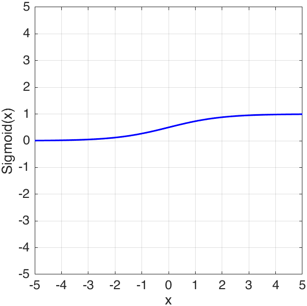
Sigmoid activation function
The Sigmoid activation function is:
\[\sigma(x)=\dfrac{1}{1+e^{-x}}\]we could calculate it using MATLAB sigmoid function1:
1
2
3
4
5
6
7
8
9
10
11
x = dlarray(-5:0.1:5);

figure("Color","w")
nexttile
hold(gca,"on"),box(gca,"on"),grid(gca,"on")
set(gca,"DataAspectRatio",[1,1,1],"FontSize",12)
plot(x,sigmoid(x),"LineWidth",1.5,"Color","b")
xlabel("x")
ylabel("Sigmoid(x)")
xticks(-5:5)
ylim([-5,5])
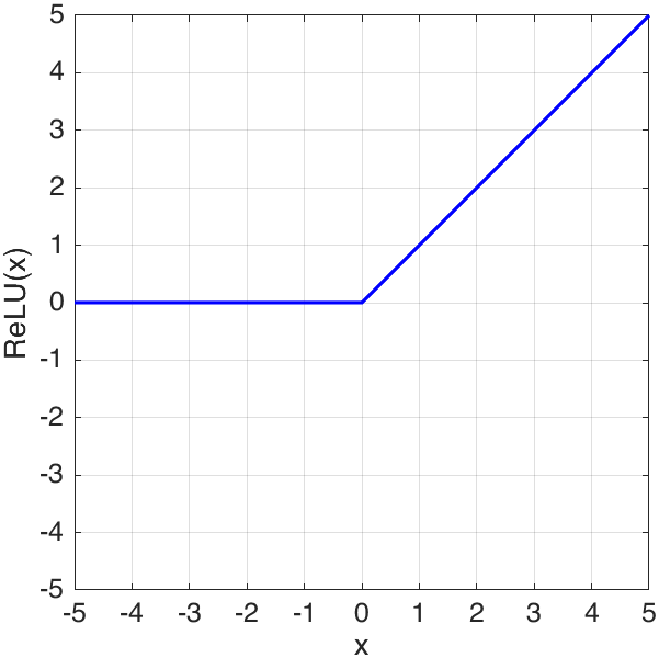
ReLU activation function (Rectified Linear Unit)
The ReLU (Rectified Linear Unit) activation function is:
\[f(x)=\left\{\begin{split} x,\ & x>0\\ 0,\ & x\le0\\ \end{split}\right.\]we could calculate it using relu function2:
1
2
3
4
5
6
7
8
9
10
11
x = dlarray(-5:0.1:5);

figure("Color","w")
nexttile
hold(gca,"on"),box(gca,"on"),grid(gca,"on")
set(gca,"DataAspectRatio",[1,1,1],"FontSize",12)
plot(x,relu(x),"LineWidth",1.5,"Color","b")
xlabel("x")
ylabel("ReLU(x)")
xticks(-5:5)
ylim([-5,5])
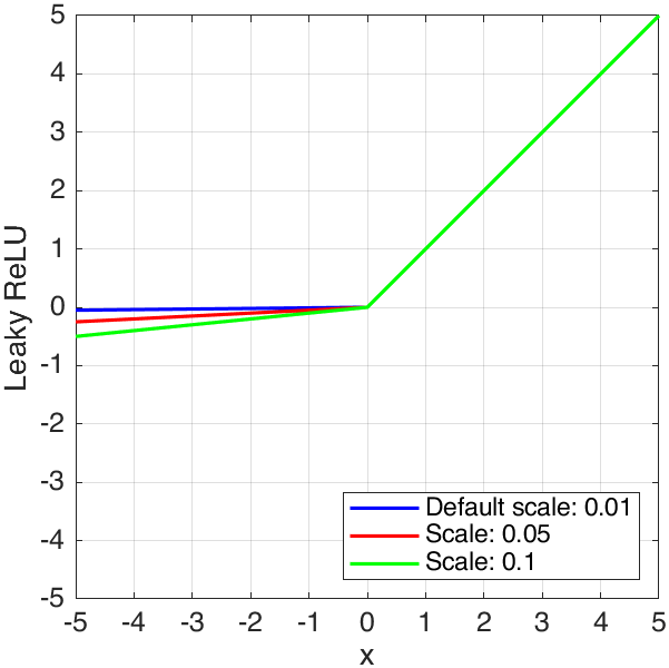
Leaky ReLU activation function
The Leaky ReLU activation function is:
\[f(x)=\left\{\begin{split} &x,\ & x>0\\ &\text{scale}\times x,\ & x\le0\\ \end{split}\right.\]where $\text{scale}$ is scale factor of Leaky ReLU. We could calculate it using leakyrelu function3:
1
2
3
4
5
6
7
8
9
10
11
12
13
14
x = dlarray(-5:0.1:5);

figure("Color","w")
nexttile
hold(gca,"on"),box(gca,"on"),grid(gca,"on")
set(gca,"DataAspectRatio",[1,1,1],"FontSize",12)
plot(x,leakyrelu(x),"LineWidth",1.5,"Color","b","DisplayName","Default scale: 0.01")
plot(x,leakyrelu(x,0.05),"LineWidth",1.5,"Color","r","DisplayName","Scale: 0.05")
plot(x,leakyrelu(x,0.1),"LineWidth",1.5,"Color","g","DisplayName","Scale: 0.1")
xlabel("x")
ylabel("Leaky ReLU")
xticks(-5:5)
ylim([-5,5])
legend("Location","southeast")
Gaussian error linear unit activation function (GELU)
The GELU (Gaussian error linear unit) activation function is4:
\[\text{GELU}(x)=\dfrac{x}2\big(1+\mathrm{erf}(\dfrac{x}{\sqrt{2}})\big)\]where $\text{erf}(x)$ is the error function:
\[\text{erf}(x)=\dfrac2{\sqrt\pi}\int_0^x\mathrm{e}^{-t^2}\mathrm{d}t\]we could calculate it using gelu function4. Besides, tanh method can be used to approximate $\text{erf}(x)$ by specifying "Approximation" property of gelu function as "tanh":
1
2
3
4
5
6
7
8
9
10
11
12
13
x = dlarray(-5:0.1:5);

figure("Color","w")
nexttile
hold(gca,"on"),box(gca,"on"),grid(gca,"on")
set(gca,"DataAspectRatio",[1,1,1],"FontSize",12)
plot(x,gelu(x),"LineWidth",1.5,"Color","b","DisplayName","Approximation method (default): none")
plot(x,gelu(x,"Approximation","tanh"),"LineWidth",1.5,"Color","r","DisplayName","Approximation method: tanh")
xlabel("x")
ylabel("GELU")
xticks(-5:5)
ylim([-5,5])
legend("Location","southeast")
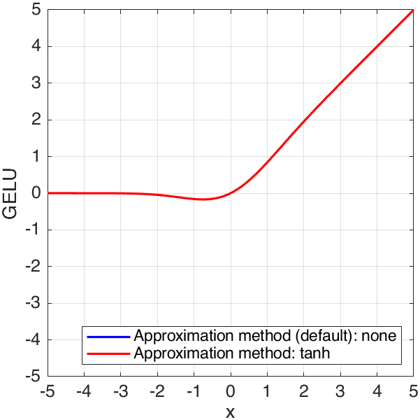
As can be seen, the output values are not significantly different regardless of whether approximation method "tanh" is used or not. I guess maybe the function of approximation is to save computation time.
And note that, gelu function is only available from MATLAB R2022b version.
tanh activation function (Heperbolic tangent)
The tanh activation function is:
\[\text{tanh}(x)=\dfrac{\text{sinh}(x)}{\text{cosh}(x)}=\dfrac{\mathrm{e}^{2x}-1}{\mathrm{e}^{2x}+1}\]where $\text{sinh}(x)$ is hyperbolic sine5:
\[\text{cosh}(x)=\dfrac{\mathrm{e}^{x}-\mathrm{e}^{-x}}{2}\]and $\text{cosh}(x)$ is hyperbolic cosine6:
\[\text{cosh}(x)=\dfrac{\mathrm{e}^{x}+\mathrm{e}^{-x}}{2}\]we could calculate it using gelu function7:
1
2
3
4
5
6
7
8
9
10
11
x = dlarray(-5:0.1:5);

figure("Color","w")
nexttile
hold(gca,"on"),box(gca,"on"),grid(gca,"on")
set(gca,"DataAspectRatio",[1,1,1],"FontSize",12)
plot(x,tanh(x),"LineWidth",1.5,"Color","b")
xlabel("x")
ylabel("tanh(x)")
xticks(-5:5)
ylim([-5,5])
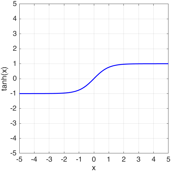
By the way, not like other activation functions aforementioned, tanh function is not provided by MATLAB Deep Learning Toolbox, but from basic MATLAB Mathematics, so it is not necessary to convert input to dlarray data type.
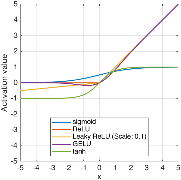
Contrast above activation functions
1
2
3
4
5
6
7
8
9
10
11
12
13
14
15
16
17
x = dlarray(-5:0.1:5);

figure("Color","w")
nexttile
hold(gca,"on"),box(gca,"on"),grid(gca,"on")
set(gca,"DataAspectRatio",[1,1,1],"FontSize",12)
plot(x,sigmoid(x),"LineWidth",1.5,"DisplayName","sigmoid")
plot(x,relu(x),"LineWidth",1.5,"DisplayName","ReLU")
plot(x,leakyrelu(x,0.1), ...
    "LineWidth",1.5,"DisplayName","Leaky ReLU (Scale: 0.1)")
plot(x,gelu(x),"LineWidth",1.5,"DisplayName","GELU")
plot(x,tanh(x),"LineWidth",1.5,"DisplayName","tanh")
xlabel("x")
ylabel("Activation value")
xticks(-5:5)
ylim([-5,5])
legend("Location","south")
References