Construct and Train the Network with Multiple Outputs in MATLAB

Feb. 27, 2024

Introduction

The MATLAB official example, “Train Network with Multiple Outputs ” ¹, shows how to construct a multi-output neural network using custom training loop.

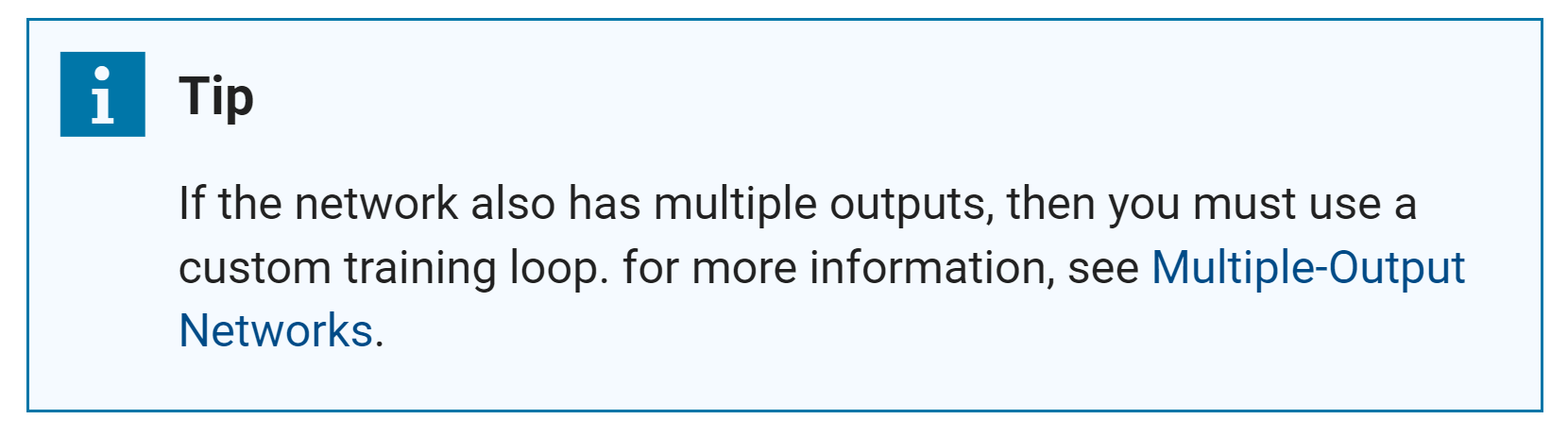
Actually, as mentioned in the official documentation, “Multiple-Input and Multiple-Output Networks”², if the constructed network has multiple outputs, using custom training loop is the only choice, that is trainNetwork function is not available:

It is a good example shows how to construct neural networks to solve multi-label problems in MATLAB. Therefore, I would record it down in this post and make some notes about it.

Reproduce the example: train and test the network

Specifically, this example is to show “how to train a deep learning network with multiple outputs that predict both labels and angles of rotations of handwritten digits”¹. And the necessary code for preparing training data set, constructing and training the network shows as follows:

clc,clear,close all
rng("default")

% Load training data
[XTrain,T1Train,T2Train] = digitTrain4DArrayData;

dsXTrain = arrayDatastore(XTrain,IterationDimension=4);
dsT1Train = arrayDatastore(T1Train);
dsT2Train = arrayDatastore(T2Train);

dsTrain = combine(dsXTrain,dsT1Train,dsT2Train);

classNames = categories(T1Train);
numClasses = numel(classNames);
numObservations = numel(T1Train);

% Define deep learning model
% Define the main block of layers as a layer graph.
layers = [
    imageInputLayer([28 28 1],Normalization="none")

    convolution2dLayer(5,16,Padding="same")
    batchNormalizationLayer
    reluLayer(Name="relu_1")

    convolution2dLayer(3,32,Padding="same",Stride=2)
    batchNormalizationLayer
    reluLayer
    convolution2dLayer(3,32,Padding="same")
    batchNormalizationLayer
    reluLayer

    additionLayer(2,Name="add")

    fullyConnectedLayer(numClasses)
    softmaxLayer(Name="softmax")];

lgraph = layerGraph(layers);

% And the skip connection
layers = [
    convolution2dLayer(1,32,Stride=2,Name="conv_skip")
    batchNormalizationLayer
    reluLayer(Name="relu_skip")];

lgraph = addLayers(lgraph,layers);
lgraph = connectLayers(lgraph,"relu_1","conv_skip");
lgraph = connectLayers(lgraph,"relu_skip","add/in2");

% Add the fully connected layer for regression.
layers = fullyConnectedLayer(1,Name="fc_2");
lgraph = addLayers(lgraph,layers);
lgraph = connectLayers(lgraph,"add","fc_2");

% Create a dlnetwork object from the layer graph.
net = dlnetwork(lgraph);

% Specify Training Options
numEpochs = 30;
miniBatchSize = 128;

% Train the network
mbq = minibatchqueue(dsTrain,...
    MiniBatchSize=miniBatchSize,...
    MiniBatchFcn=@preprocessData,...
    MiniBatchFormat=["SSCB" "" ""]);

% Initialize the training progress plot.
figure("Color","w")
hold(gca,"on"),box(gca,"on"),grid(gca,"on")
C = colororder;
lineLossTrain = animatedline("Color",C(2,:));
ylim([0 inf])
xlabel("Iteration")
ylabel("Loss")

% Initialize parameters for Adam.
trailingAvg = [];
trailingAvgSq = [];

% Train the model
iteration = 0;
start = tic;

% Loop over epochs.
for epoch = 1:numEpochs

    % Shuffle data.
    shuffle(mbq)

    % Loop over mini-batches
    while hasdata(mbq)

        iteration = iteration + 1;

        [X,T1,T2] = next(mbq);

        % Evaluate the model loss, gradients, and state using
        % the dlfeval and modelLoss functions.
        [loss,gradients,state] = dlfeval(@modelLoss,net,X,T1,T2);
        net.State = state;

        % Update the network parameters using the Adam optimizer.
        [net,trailingAvg,trailingAvgSq] = adamupdate(net,gradients, ...
            trailingAvg,trailingAvgSq,iteration);

        % Display the training progress.
        D = duration(0,0,toc(start),Format="hh:mm:ss");
        loss = double(loss);
        addpoints(lineLossTrain,iteration,loss)
        title("Epoch: " + epoch + ", Elapsed: " + string(D))
        drawnow
    end
end
% Copyright 2019 The MathWorks, Inc.

where model loss function modelLoss and mini-batch preprocessing function preprocessData are respectively:

% Define model loss function
function [loss,gradients,state] = modelLoss(net,X,T1,T2)
[Y1,Y2,state] = forward(net,X,Outputs=["softmax" "fc_2"]);

lossLabels = crossentropy(Y1,T1);
lossAngles = mse(Y2,T2);

loss = lossLabels + 0.1*lossAngles;
gradients = dlgradient(loss,net.Learnables);
end

% Define mini-batch preprocessing function
function [X,T1,T2] = preprocessData(dataX,dataT1,dataT2)
% Extract image data from cell and concatenate
X = cat(4,dataX{:});

% Extract label data from cell and concatenate
T1 = cat(2,dataT1{:});

% Extract angle data from cell and concatenate
T2 = cat(2,dataT2{:});

% One-hot encode labels
T1 = onehotencode(T1,1);
end

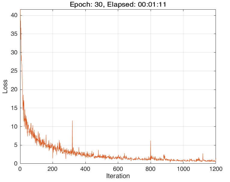
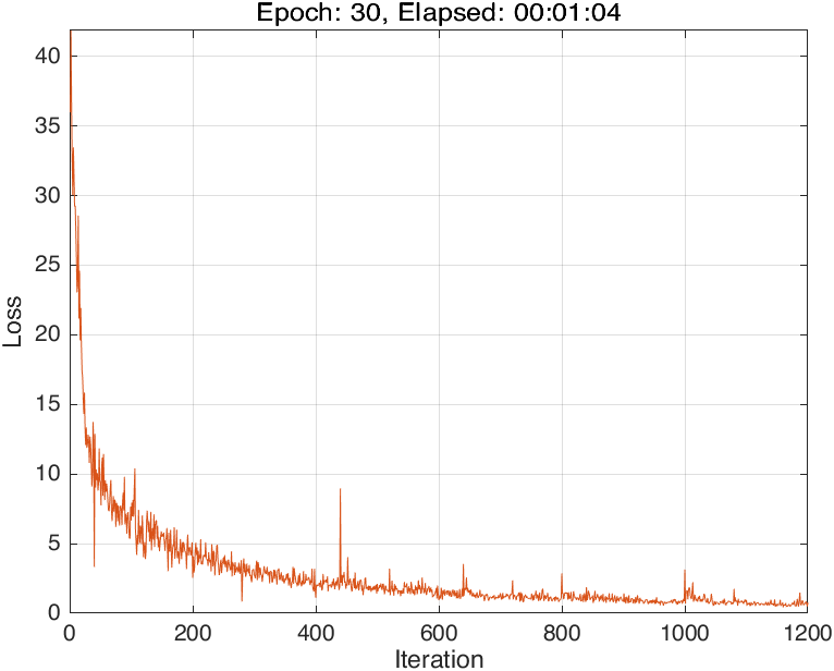
The training progress of running Script 1 looks like:

and we could evaluate the well-trained neural network using the following script:

% Load test data set
[XTest,T1Test,T2Test] = digitTest4DArrayData;

dsXTest = arrayDatastore(XTest,IterationDimension=4);
dsT1Test = arrayDatastore(T1Test);
dsT2Test = arrayDatastore(T2Test);

dsTest = combine(dsXTest,dsT1Test,dsT2Test);

mbqTest = minibatchqueue(dsTest,...
    MiniBatchSize=miniBatchSize,...
    MiniBatchFcn=@preprocessData,...
    MiniBatchFormat=["SSCB" "" ""]);

classesPredictions = [];
anglesPredictions = [];
classCorr = [];
angleDiff = [];

% Loop over mini-batches.
while hasdata(mbqTest)

    % Read mini-batch of data.
    [X,T1,T2] = next(mbqTest);

    % Make predictions using the predict function.
    [Y1,Y2] = predict(net,X,Outputs=["softmax" "fc_2"]);

    % Determine predicted classes.
    Y1 = onehotdecode(Y1,classNames,1);
    classesPredictions = [classesPredictions Y1]; %#ok

    % Dermine predicted angles
    Y2 = extractdata(Y2);
    anglesPredictions = [anglesPredictions Y2]; %#ok

    % Compare predicted and true classes
    T1 = onehotdecode(T1,classNames,1);
    classCorr = [classCorr Y1 == T1]; %#ok

    % Compare predicted and true angles
    angleDiffBatch = Y2 - T2;
    angleDiffBatch = extractdata(gather(angleDiffBatch));
    angleDiff = [angleDiff angleDiffBatch]; %#ok
end

% Evaluate the classification accuracy.
accuracy = mean(classCorr);

% Evaluate the regression accuracy
angleRMSE = sqrt(mean(angleDiff.^2));


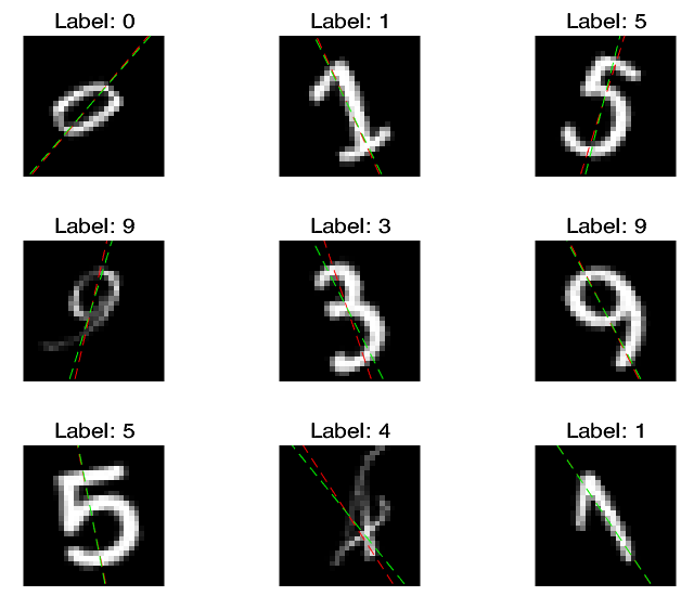
% View some of the images with their predictions. 
% Display the predicted angles in red and the correct labels in green.
idx = randperm(size(XTest,4),9);
figure("Color","w")
for i = 1:9
    subplot(3,3,i)
    I = XTest(:,:,:,idx(i));
    imshow(I)
    hold on

    sz = size(I,1);
    offset = sz/2;

    thetaPred = anglesPredictions(idx(i));
    plot(offset*[1-tand(thetaPred) 1+tand(thetaPred)],[sz 0],"r--")

    thetaValidation = T2Test(idx(i));
    plot(offset*[1-tand(thetaValidation) 1+tand(thetaValidation)],[sz 0],"g--")

    hold off
    label = string(classesPredictions(idx(i)));
    title("Label: " + label)
end
% Copyright 2019 The MathWorks, Inc.

The two measures indicating the model performance, accuracy for classification task and angleRMSE for regression task, are:

>> accuracy, angleRMSE
accuracy =
    0.9792

angleRMSE =
  single
    6.8784

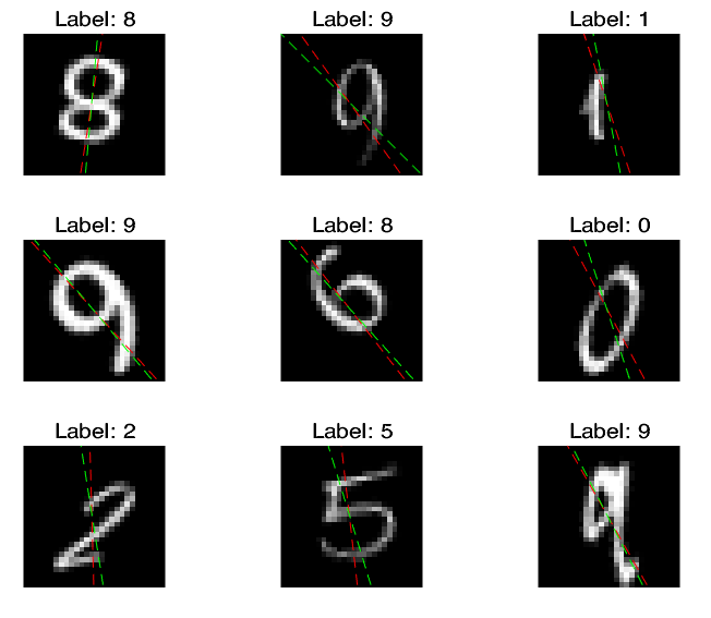
where the green lines represent the true angles, and red lines represent the predicted angles.

Discussions

Prepare data sets

In Script 1, we use the following code to prepare training data set for training the network (so do for preparing test data set in Script 2):

% Load training data
[XTrain,T1Train,T2Train] = digitTrain4DArrayData;

dsXTrain = arrayDatastore(XTrain,IterationDimension=4);
dsT1Train = arrayDatastore(T1Train);
dsT2Train = arrayDatastore(T2Train);

dsTrain = combine(dsXTrain,dsT1Train,dsT2Train);

where the data type of XTrain (greyscale image), T1Train (labels for classification), T2Train (labels for regression) is clear:

>> whos XTrain T1Train T2Train
  Name            Size                      Bytes  Class          Attributes

  T1Train      5000x1                        6062  categorical              
  T2Train      5000x1                       40000  double                   
  XTrain         28x28x1x5000            31360000  double         

After importing them, we should use arrayDatastore function³ and combine function⁴ to prepare data set for training:

dsXTrain = arrayDatastore(XTrain,IterationDimension=4);
dsT1Train = arrayDatastore(T1Train);
dsT2Train = arrayDatastore(T2Train);

dsTrain = combine(dsXTrain,dsT1Train,dsT2Train);

The default value of IterationDimension property of arrayDatastore function is 1. Easily speaking, the value of IterationDimension property specifies which dimension MATLAB should count the sample size along.

By the way, data actually aren’t stored in variables dsXTrain, dsT1Train, and dsT2Train:

>> whos dsXTrain dsT1Train dsT2Train
  Name           Size            Bytes  Class                                 Attributes

  dsT1Train      1x1                 8  matlab.io.datastore.ArrayDatastore              
  dsT2Train      1x1                 8  matlab.io.datastore.ArrayDatastore              
  dsXTrain       1x1                 8  matlab.io.datastore.ArrayDatastore              

arrayDatastore seemingly just defines how to read data from in-memory variables XTrain, T1Train, and T2Train³. And so do for dsTrain, which is created by combine function⁴:

>> whos dsTrain
  Name         Size            Bytes  Class                                    Attributes

  dsTrain      1x1                 8  matlab.io.datastore.CombinedDatastore              

To sum up, the whole preparation work is showed as above, and we finally could obtain variable dsTrain, which will be put into minibatchqueue function to create mini-batch.

Neural network structure

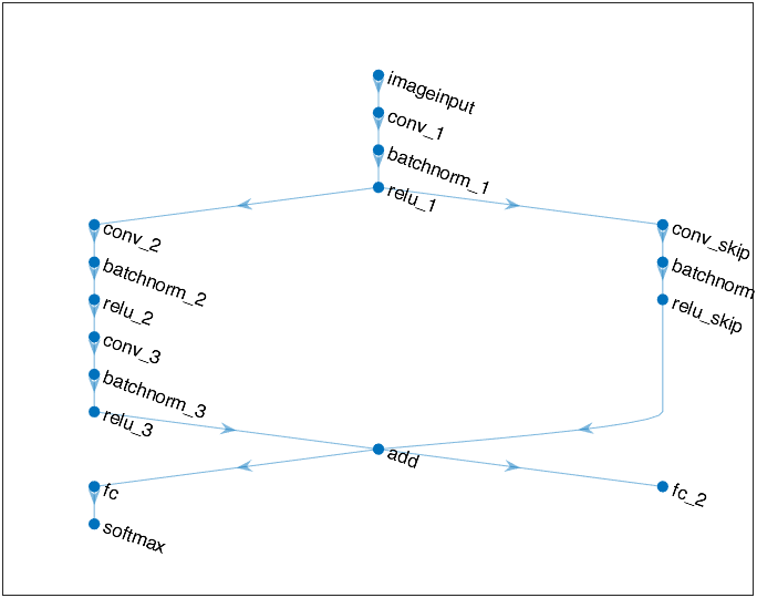
We could use plot(lagraph) or built-in function analyzeNetwork⁵ to inspect the neural network structure:

plot(lgraph)

analyzeNetwork(net)

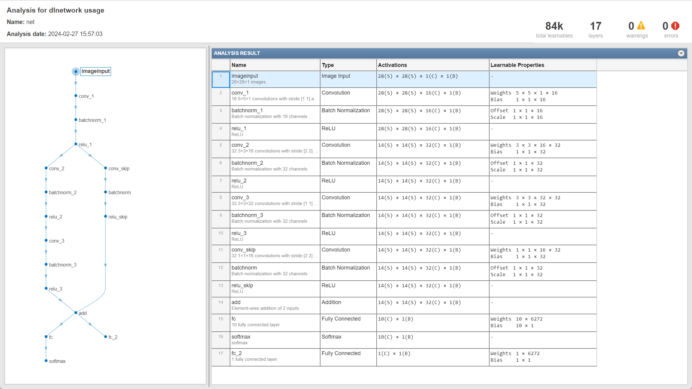
As can be seen, when creating the main block of layers in Script 1, an addition layer is created by additionLayer function⁶ before creating the last fully-connected layer. Then, a skip connection is then connected to the main branch by addLayers⁷and connectLayers⁸ (In fact, as will be showed in Appendix I, this skip connection is not necessary.)

It should be noted that, if we want to train the neural network using custom training loop, we don’t need to use classificationLayer or regressionLayer to create the output layer as we do when using trainNetwork function to train (as in references ⁹ and ¹⁰, respectively). Instead, using softmaxLayer and fullyConnectedLayer to create the output layers and followed by loss calculation is enough.

Model loss function

As mentioned above, the loss value of neural network is calculated by modelLoss function, and the total loss consists of two parts:

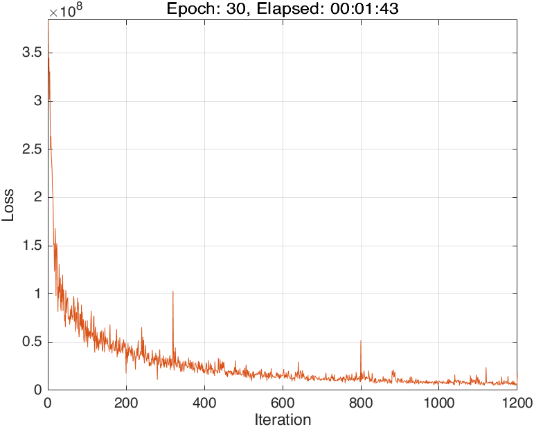
\[\text{Loss}=\text{Cross-entropy}(Y_1,T_1)+0.1\times\text{MSE}(Y_2,T_2)\label{eq1}\]

Although the official documentation¹ doesn’t explain the function of coefficient $0.1$, I guess it is used to balance two loss value and therefore balance two different tasks (Note that this is just my guess, and in fact, if we expand the gap between them to an extreme situation, the result is still good. See Appendix II.). If we modify modelLoss function to make it output two loss values, we could plot how the loss values change as iteration:

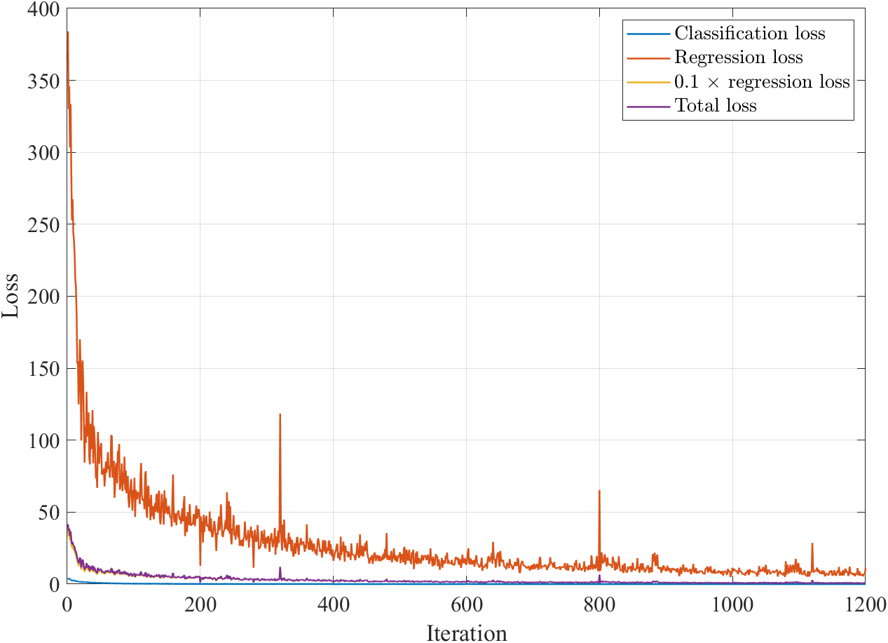
As can be seen, the classification loss, $\text{Cross-entropy}(Y_1,T_1)$, is rather less than the regression regression loss, $\text{MSE}(Y_2,T_2)$, and multiplying $0.1$ before the latter narrows the gap between them.

Appendix

Appendix I

The figure of network architecture may cause a false feeling, that is the main part of the network (the left branch) is for classification, and the right one is for regression:

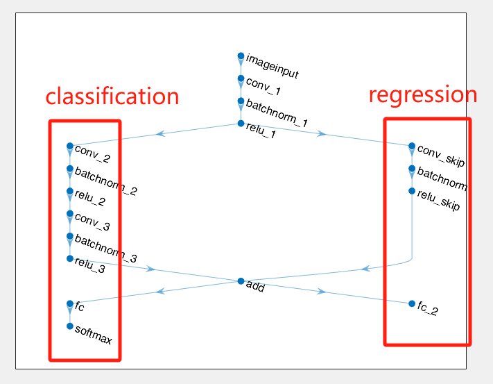
However, it is a wrong understanding! For example, if we delete the right branch, and the network architecture at this time is like:

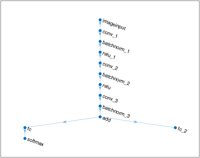
and it also has a good performance:

>> accuracy,angleRMSE
accuracy =
    0.9810

angleRMSE =
  single
    6.0480

So, to my mind, the reason a neural network is called multi-output is that it has multiple output layers and different output layers correspond to different loss function calculation methods. In this example, no matter how complex the structure of hidden layers or how many branches it has, in the backward process, the learnable parameters of each layer are optimized by derivating the total loss value which is calculated by $\eqref{eq1}$. In fact, if classification loss and regression loss are derivated for different network branches, then this method is not fundamentally different from establishing two separate neural networks.

Appendix II

Here, I will change the weights of two loss values of modelLoss function to:

\[\text{Loss}=10^{-6}\times\text{Cross-entropy}(Y_1,T_1)+10^{6}\times\text{MSE}(Y_2,T_2)\]

that is:

% Define the modified model loss function
function [loss,gradients,state,lossLabels,lossAngles] = modelLoss_modified(net,X,T1,T2)
[Y1,Y2,state] = forward(net,X,Outputs=["softmax" "fc_2"]);

lossLabels = crossentropy(Y1,T1);
lossAngles = mse(Y2,T2);

loss = 1e-6*lossLabels + 1e6*lossAngles;
gradients = dlgradient(loss,net.Learnables);
end

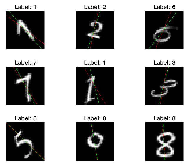
In this case, the training progress plot is like:

I expect the classification effect of the network is extremely bad, but the result shows that I am wrong:

>> accuracy,angleRMSE
accuracy =
    0.9752
    
angleRMSE =
  single
    8.8155

Therefore, I am not that sure what the role of coefficient $0.1$ in $\eqref{eq1}$ right now.

References