Animate Linear Transformation and Affine Transformation

Dec. 02, 2023

Animation of linear transformation

Two-dimensional vector space

Angelo Yeo uploaded his two works to the “MATLAB Flipbook Mini Hack” contest ¹ ², showing how to animate the continuous process of a specific linear transformation. The first one ¹ shows the linear transformation imposed by matrix:

\[A=\begin{bmatrix} 0 & 1\\ 1 & 0\\ \end{bmatrix}\label{eq1}\]

animation

clc,clear,close all

contestAnimator()

function contestAnimator()
animFilename = "animation.gif";
firstFrame = true;
framesPerSecond = 24;
delayTime = 1/framesPerSecond;

for frame = 1:48
    drawframe(frame)
    fig = gcf();
    fig.Units = "pixels";
    fig.Position(3:4) = [300,300];
    im = getframe(fig);
    [A,map] = rgb2ind(im.cdata,256);
    if firstFrame
        firstFrame = false;
        imwrite(A,map,animFilename, LoopCount=Inf, DelayTime=delayTime);
    else
        imwrite(A,map,animFilename, WriteMode="append", DelayTime=delayTime);
    end
end
end

function drawframe(f)
cla
mtx2apply = [0, 1; 1, 0];
vu = ones(2, 9) * 4;
vu(1,:) = -4:4;
vd = ones(2, 9) * (-4);
vd(1,:) = -4:4;
hl = ones(2, 9) * (-4);
hl(2,:) = -4:4;
hr = ones(2, 9) * 4;
hr(2,:) = -4:4;
setBasicCanvas(vu, vd, hl, hr);
mtx4vis = eye(2) + (mtx2apply - eye(2)) * ((f-1)/(48-1));
hv = plotLines(mtx4vis * vu, mtx4vis * vd, [109, 155, 222]/255);
hh = plotLines(mtx4vis * hl, mtx4vis * hr, [109, 155, 222]/255);
ha1 = drawArrow([0, 0], mtx4vis * [1; 0], "r");
ha2 = drawArrow([0, 0], mtx4vis * [0; 1], "g");
function setBasicCanvas(vu, vd, hl, hr)
    set(gcf,'color','k')
    ax = newplot;
    daspect(ax, [1,1,1])
    set(ax, 'position', [0 0 1 1], 'visible', 'off')
    xlim([-4, 4])
    ylim([-4, 4])
    plotLines(vu, vd);
    plotLines(hl, hr);
end
function h = drawArrow(p1, p2, color)
    dp = p2 - p1;
    hold on;
    h = quiver(p1(1), p1(2) ,dp(1), dp(2), 0, "filled", "Color", color, "linewidth", 2, "MaxHeadSize", 0.5);
end
function h = plotLines(v1, v2, color)
    if nargin<3
        color = ones(1,3) * 0.3;
    end
    assert(length(v1) == length(v2), "The two input vectors must have same length!")
    for i = 1:length(v1)
        h(i) = line([v1(1, i), v2(1, i)], [v1(2, i), v2(2, i)], 'color', color, 'linewidth',1);
    end
end
end

Another work ² shows the linear transformation:

\[A=\begin{bmatrix} 2 & 1\\ 1 & 2\\ \end{bmatrix}\label{eq2}\]

animation

clc,clear,close all

contestAnimator()

function contestAnimator()
animFilename = "animation.gif";
firstFrame = true;
framesPerSecond = 24;
delayTime = 1/framesPerSecond;

for frame = 1:48
    drawframe(frame)
    fig = gcf();
    fig.Units = "pixels";
    fig.Position(3:4) = [300,300];
    im = getframe(fig);
    [A,map] = rgb2ind(im.cdata,256);
    if firstFrame
        firstFrame = false;
        imwrite(A,map,animFilename, LoopCount=Inf, DelayTime=delayTime);
    else
        imwrite(A,map,animFilename, WriteMode="append", DelayTime=delayTime);
    end
end
end

function drawframe(f)
cla
mtx2apply = [2, 1; 1, 2];
vu = ones(2, 9) * 4;
vu(1,:) = -4:4;
vd = ones(2, 9) * (-4);
vd(1,:) = -4:4;
hl = ones(2, 9) * (-4);
hl(2,:) = -4:4;
hr = ones(2, 9) * 4;
hr(2,:) = -4:4;

setBasicCanvas(vu, vd, hl, hr);
mtx4vis = eye(2) + (mtx2apply - eye(2)) * ((f-1)/(48-1));
hv = plotLines(mtx4vis * vu, mtx4vis * vd, [109, 155, 222]/255);
hh = plotLines(mtx4vis * hl, mtx4vis * hr, [109, 155, 222]/255);
ha1 = drawArrow([0, 0], mtx4vis * [1; 0], "r");
ha2 = drawArrow([0, 0], mtx4vis * [0; 1], "g");
    function setBasicCanvas(vu, vd, hl, hr)
        set(gcf,'color','k')
        ax = newplot;
        daspect(ax, [1,1,1])
        set(ax, 'position', [0 0 1 1], 'visible', 'off')
        xlim([-4, 4])
        ylim([-4, 4])
        plotLines(vu, vd);
        plotLines(hl, hr);
    end
    function h = drawArrow(p1, p2, color)
        dp = p2 - p1;
        hold on;
        h = quiver(p1(1), p1(2) ,dp(1), dp(2), 0, "filled", "Color", color, "linewidth", 2, "MaxHeadSize", 0.5);
    end
    function h = plotLines(v1, v2, color)
        if nargin<3
            color = ones(1,3) * 0.3;
        end
        assert(length(v1) == length(v2), "The two input vectors must have same length!")
        for i = 1:length(v1)
            h(i) = line([v1(1, i), v2(1, i)], [v1(2, i), v2(2, i)], 'color', color, 'linewidth',1);
        end
    end
end

These two works are basically the same, and the only difference is that mtx2apply in drawframe function, i.e., the matrix corresponding linear transformation, is different.

In general, the self-defined drawframe function used to generate each frame draws three parts of content in the frame:

(1) The fixed gray grid lines in the background;

(2) The animated blue grid lines;

(3) The two animated basis vectors, the green one and red one;

By the way, these two .gif files show the characteristics of linear transformation ³ ⁴: (a) remains the origin, (b) keep the grid lines remain parallel and evenly spaced, and (c) the columns of matrix can be interpreted as the two special vectors where the basis vectors of vector space after transformation land.

As can be seen from dfrawframe function, the animated grid lines and vectors in the $i$-th frame is determined by multiplying the matrix $A^\prime$:

\[A^\prime=\mathrm{I}+\dfrac{i-1}{n-1}(A-\mathrm{I}),\ i\in[1,n]\label{eq3}\]

where $\mathrm{I}$ is $2$-order identity matrix (corresponds two-dimensional vector space), $A$ is the matrix corresponding to the applied linear transformation. And $A^\prime$ in $\eqref{eq3}$ can be rewritten as:

\[A^\prime=\dfrac{n-i}{n-1}\mathrm{I}+\dfrac{i-1}{n-1}A\]

which means that $A^\prime$ is the weighted average of $\mathrm{I}$ and $A$, and:

\[A^\prime=\left\{ \begin{split} \mathrm{I},\ &\text{if }i=1\\ A,\ &\text{if }i=n\\ \end{split}\right.\]

When I ever watched the 3Blue1Brown’s videos showing the relationship between the matrix and the linear transformation ⁴, I was curious about how to animate the whole process of linear transformation, so these two works of Angelo Yeo give me the answer.

Three-dimensional vector space

But, to take things to step further, how to show this animation process in the tree-dimensional space? Actually, it is easy to show the transformation of basis vectors, but the construction and animation of grid lines in three-dimensional space are kind of difficult.

In Angelo Yeo’s code, he defines the grid lines by the following code:

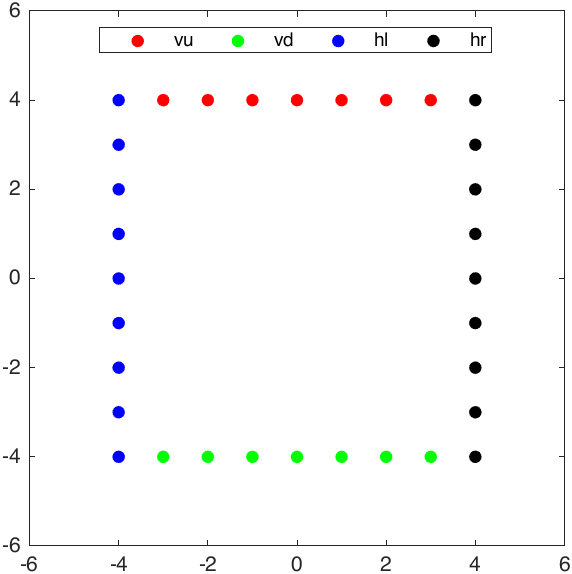
vu = ones(2, 9) * 4;
vu(1,:) = -4:4;
vd = ones(2, 9) * (-4);
vd(1,:) = -4:4;
hl = ones(2, 9) * (-4);
hl(2,:) = -4:4;
hr = ones(2, 9) * 4;
hr(2,:) = -4:4;

As can be seen, each column vector of vu, vd is respectively the coordinates of upper end point and lower end point of the vertical grid lines, and each column vector of hl and hr is respectively the coordinates of left end point and right end point of the horizontal grid lines:

......
hold(gca,"on"),box(gca,"on")
daspect(gca,[1,1,1])
axis([-6,6,-6,6])
scatter(vu(1,:),vu(2,:), ...
    "filled","r","DisplayName","vu")
scatter(vd(1,:),vd(2,:), ...
    "filled","g","DisplayName","vd")
scatter(hl(1,:),hl(2,:),"filled","b", ...
    "DisplayName","hl")
scatter(hr(1,:),hr(2,:),"filled","k", ...
    "DisplayName","hr")
legend("Location","north","Orientation","horizontal");

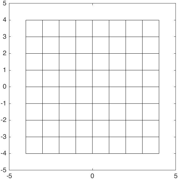
This method of creating grid lines is clear, but it is difficult to generalize to the three-dimensional vector space. So, I use MATLAB meshgrid function to generate the coordinates of each grid point, and then extract the coordinates of grid end points, to draw the grid lines:

clc,clear,close all

[x,y] = meshgrid(-4:1:4);
beginningPoints = [[x(:,1);x(1,:)'],[y(:,1);y(1,:)']];
endingPoints = [[x(:,end);x(end,:)'],[y(:,end);y(end,:)']];

box(gca,"on")
daspect(gca,[1,1,1])
axis(5*[-1,1,-1,1])

for i = 1:height(beginningPoints)
    line([beginningPoints(i,1),endingPoints(i,1)], ...
        [beginningPoints(i,2),endingPoints(i,2)],"Color","k")
end

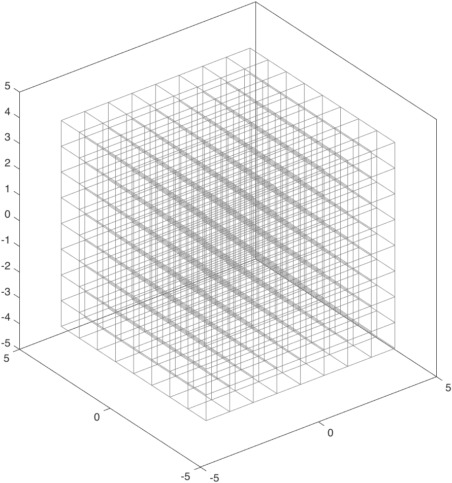
By a similar way, we could draw the grid lines in the three-dimensional vector space:

clc,clear,close all

[x,y,z] = meshgrid(-4:4);

figure("Position",[708.33,503.67,865.33,720.67])
hold(gca,"on"),box(gca,"on")
view(3)
axis(5*[-1,1,-1,1,-1,1])
daspect(gca,[1,1,1])

beginningPoints = [];
enddingPoints = [];

% 1-2
for i = 1:size(x,1)
    for j = 1:size(x,2)
        beginningPoints = [beginningPoints;x(i,j,1),y(i,j,1),z(i,j,1)]; %#ok
        enddingPoints = [enddingPoints;x(i,j,end),y(i,j,end),z(i,j,end)]; %#ok
    end
end

% 1-3
for i = 1:size(x,1)
    for j = 1:size(x,3)
        beginningPoints = [beginningPoints;x(i,1,j),y(i,1,j),z(i,1,j)]; %#ok
        enddingPoints = [enddingPoints;x(i,end,j),y(i,end,j),z(i,end,j)]; %#ok
    end
end

% 2-3
for i = 1:size(x,2)
    for j = 1:size(x,3)
        beginningPoints = [beginningPoints;x(1,i,j),y(1,i,j),z(1,i,j)]; %#ok
        enddingPoints = [enddingPoints;x(end,i,j),y(end,i,j),z(end,i,j)]; %#ok
    end
end

for i = 1:height(beginningPoints)
    plot3([beginningPoints(i,1),enddingPoints(i,1)], ...
        [beginningPoints(i,2),enddingPoints(i,2)], ...
        [beginningPoints(i,3),enddingPoints(i,3)], ...
        "Color",[0.5,0.5,0.5],"LineWidth",0.1)
end

And therefore, we could animate the linear transformation process in the three-dimensional vector space by the following code:

clc,clear,close all

contestAnimator()

function contestAnimator()
animFilename = "gif.gif";
fps = 24;

for frame = 1:48
    drawframe(frame)
    fig = gcf();
    im = getframe(fig);
    [A,map] = rgb2ind(im.cdata,256);
    if frame == 1
        imwrite(A,map,animFilename,"LoopCount",Inf,"DelayTime",1/fps);
    elseif frame ~= 48
        imwrite(A,map,animFilename,"WriteMode","append","DelayTime",1/fps);
    else
        for i = 1:24
            imwrite(A,map,animFilename,"WriteMode","append","DelayTime",1/fps);
        end
    end
end
end

function drawframe(f)
cla
set(gcf,"Color","k","Position",[693.67,281.67,1146,956.67])
ax = gca();
hold(ax,"on"),axis(ax,"off")
ax.Toolbar.Visible = "off";
daspect(ax,[1,1,1])
view(ax,3)
axis([-4,4,-4,4,-4,4])

% Calculate matrix
matrix = [0,1,0;0,0,1;1,0,0];
mtx4vis = eye(3)+(matrix-eye(3))*((f-1)/(48-1));

% Obtain the end points of grid lines
[x,y,z] = meshgrid(-4:2:4);
beginningPoints = [];
endingPoints = [];
% 1-3
for i = 1:size(x,1)
    for j = 1:size(x,3)
        beginningPoints = [beginningPoints;x(1,i,j),y(1,i,j),z(1,i,j)]; %#ok
        endingPoints = [endingPoints;x(end,i,j),y(end,i,j),z(end,i,j)]; %#ok
    end
end
% 1-2
for i = 1:size(x,1)
    for j = 1:size(x,2)
        beginningPoints = [beginningPoints;x(i,j,1),y(i,j,1),z(i,j,1)]; %#ok
        endingPoints = [endingPoints;x(i,j,end),y(i,j,end),z(i,j,end)]; %#ok
    end
end
% 2-3
for i = 1:size(x,2)
    for j = 1:size(x,3)
        beginningPoints = [beginningPoints;x(i,1,j),y(i,1,j),z(i,1,j)]; %#ok
        endingPoints = [endingPoints;x(i,end,j),y(i,end,j),z(i,end,j)]; %#ok
    end
end

% Plot fixed gray grid lines
for i = 1:height(beginningPoints)
    plot3([beginningPoints(i,1),endingPoints(i,1)], ...
        [beginningPoints(i,2),endingPoints(i,2)], ...
        [beginningPoints(i,3),endingPoints(i,3)], ...
        "Color",[0.3,0.3,0.3],"LineWidth",0.5);
end

% Plot blue animated grid lines
beginningPoints = (mtx4vis*beginningPoints')';
endingPoints = (mtx4vis*endingPoints')';
for i = 1:height(beginningPoints)
    plot3([beginningPoints(i,1),endingPoints(i,1)], ...
        [beginningPoints(i,2),endingPoints(i,2)], ...
        [beginningPoints(i,3),endingPoints(i,3)], ...
        "Color",[109,155,222]/255,"LineWidth",0.1);
end

% Plot basis vectors
basis = mtx4vis*[4,0,0;0,4,0;0,0,4];
quiver3(0,0,0,basis(1,1),basis(2,1),basis(3,1), ...
    "filled","Color","r","linewidth",2,"MaxHeadSize",0.5)
quiver3(0,0,0,basis(1,2),basis(2,2),basis(3,2), ...
    "filled","Color","g","linewidth",2,"MaxHeadSize",0.5)
quiver3(0,0,0,basis(1,3),basis(2,3),basis(3,3), ...
    "filled","Color","b","linewidth",2,"MaxHeadSize",0.5)
end

gif

Animation of affine transformation

On the other hand, a linear transformation in vector space can be viewed as a special affine transformation ⁵: “If $X$ is the point set of an affine space, then every affine transformation on $X$ can be represented as the composition of a linear transformation on $X$ and a translation of $X$. Unlike a purely linear transformation, an affine transformation need not preserve the origin of the affine space. Thus, every linear transformation is affine, but not every affine transformation is linear.” Therefore, I want to animate an affine transformation in a similar way with $\eqref{eq3}$.

Formally ⁵, in the finite-dimensional space, if the linear map is represented as a multiplication by an invertible matrix $A$ and the translation as the addition of a vector $\boldsymbol{b}$, an affine map $f$ acting on a vector $\boldsymbol{x}$ can be represented as:

\[f(\boldsymbol{x})=A\boldsymbol{x}+\boldsymbol{b}.\]

So, as a counterpart as $\eqref{eq3}$, the transformation applied on the vectors and grid lines in the $i$-th frame can be represented as:

\[\begin{split} &A^\prime_{i} = \mathrm{I}+\dfrac{i-1}{n-1}(A-\mathrm{I})\\ &\boldsymbol{b}^\prime_{i} = \dfrac{i-1}{n-1}\boldsymbol{b} \end{split},\quad i\in[1,n]\]

Two-dimensional vector space

For example, in the two-dimensional vector space, if the applied affine transformation is:

\[A=\begin{bmatrix} 1.5 & 1\\ 1 & 0\\ \end{bmatrix},\ \boldsymbol{b}=\begin{bmatrix} 1\\ 2\\ \end{bmatrix}\]

and the two vectors defined in the original vector space are:

\[\boldsymbol{v}_1=\begin{bmatrix} 2\\ 0\\ \end{bmatrix},\ \boldsymbol{v}_2=\begin{bmatrix} 0\\ 2\\ \end{bmatrix}\]

then the transformation animation can be generated by the following code:

clc,clear,close all

contestAnimator()

function contestAnimator()
animFilename = "gif.gif";
fps = 8;

for frame = 1:48
    drawframe(frame)
    fig = gcf();
    im = getframe(fig);
    [A,map] = rgb2ind(im.cdata,256);
    if frame == 1
        imwrite(A,map,animFilename,"LoopCount",Inf,"DelayTime",1/fps);
    elseif frame ~= 48
        imwrite(A,map,animFilename,"WriteMode","append","DelayTime",1/fps);
    else
        for i = 1:24
            imwrite(A,map,animFilename,"WriteMode","append","DelayTime",1/fps);
        end
    end
end
end

function drawframe(f)
cla
set(gcf,"Color","k","Position",[693.67,281.67,1146,956.67])
ax = gca();
hold(ax,"on")
axis(ax,"off")
ax.Toolbar.Visible = "off";
daspect(ax,[1,1,1])
axis(10*[-1,1,-1,1])

% Calculate matrix
rng("default")
matrix = [1.5,1;1,0];
mtx4vis = eye(2)+(matrix-eye(2))*((f-1)/(48-1));
b = [1,2]';
bprime = ((f-1)/(48-1))*b;

% Obtain the end points of grid lines
[x,y] = meshgrid(-4:1:4);
beginningPoints = [[x(:,1);x(1,:)'],[y(:,1);y(1,:)']];
endingPoints = [[x(:,end);x(end,:)'],[y(:,end);y(end,:)']];

% Plot fixed gray grid lines
for i = 1:height(beginningPoints)
    plot([beginningPoints(i,1),endingPoints(i,1)], ...
        [beginningPoints(i,2),endingPoints(i,2)], ...
        "Color",[0.3,0.3,0.3],"LineWidth",0.5);
end

% Plot blue animated grid lines
beginningPoints = (mtx4vis*beginningPoints')'+repmat(bprime',height(beginningPoints),1);
endingPoints = (mtx4vis*endingPoints')'+repmat(bprime',height(endingPoints),1);
for i = 1:height(beginningPoints)
    plot([beginningPoints(i,1),endingPoints(i,1)], ...
        [beginningPoints(i,2),endingPoints(i,2)], ...
        "Color",[109,155,222]/255,"LineWidth",0.1);
end

% Plot basis vectors
vec1 = [2;0];
vec2 = [0;2];
vec1_prime = mtx4vis*vec1+bprime;
vec2_prime = mtx4vis*vec2+bprime;

qa = plot([0,vec1_prime(1)],[0,vec1_prime(2)],...
    "Color","r","linewidth",2,"DisplayName","a","Marker",".","MarkerSize",20);
qb = plot([0,vec2_prime(1)],[0,vec2_prime(2)],...
    "Color","g","linewidth",2,"DisplayName","b","Marker",".","MarkerSize",20);

qa1 = plot([bprime(1),vec1_prime(1)],[bprime(2),vec1_prime(2)],...
    "Color","r","linewidth",2,"LineStyle","-.","DisplayName","a'","Marker",".","MarkerSize",20);
qb1 = plot([bprime(1),vec2_prime(1)],[bprime(2),vec2_prime(2)],...
    "Color","g","linewidth",2,"LineStyle","-.","DisplayName","b'","Marker",".","MarkerSize",20);

% Scatter origin
scatter(0,0,"filled","MarkerFaceColor","w")
scatter(bprime(1),bprime(2),"filled","MarkerFaceColor","w")
s = sprintf("a(%d) = [%.2f,%.2f], a'(%d) = [%.2f,%.2f], a'(%d)-A' vec1 = [%.2f,%.2f]\n", ...
    f,vec1_prime,f,vec1_prime-bprime,f,vec1_prime-bprime-mtx4vis*vec1)+...
    sprintf("b(%d) = [%.2f,%.2f], b'(%d) = [%.2f,%.2f], a'(%d)-A' vec2 = [%.2f,%.2f]\n", ...
    f,vec2_prime,f,vec2_prime-bprime,f,vec2_prime-bprime-mtx4vis*vec2);
title(s,"Color","w")
legend([qa,qb,qa1,qb1],"Location","north","Orientation","horizontal","Interpreter","tex")
end

gif

If we let $V$ denote the original vector space, and $V’$ denote the vector space after affine transformation, then we could conclude that, in the whole transformation process:

(1) The origin changes, and the red and green vectors of $V$ are NOT parallel to the animated blue grid lines;

(2) From the perspective of vector space $V^\prime$ (that is taking the changing origin as the origin): the animated blue grid lines, which are determined by the basis vectors of $V^\prime$, keep parallel and evenly spaced,or rather, the transformation applied on the vectors and grid lines are only linear transformation $A’$.

Three-dimensional vector space

Likewise, in the three-dimensional vector space, if the affine transformation is:

\[A=\begin{bmatrix} 0 & 1 & 0\\ 0 & 0 & 1\\ 1 & 0 & 0\\ \end{bmatrix},\ \boldsymbol{b}=\begin{bmatrix} 2\\1\\3 \end{bmatrix}\]

and three vectors to be transformed are:

\[\boldsymbol{v}_1 = \begin{bmatrix}2\\0\\0\end{bmatrix},\ \boldsymbol{v}_2 = \begin{bmatrix}0\\2\\0\end{bmatrix},\ \boldsymbol{v}_3 = \begin{bmatrix}0\\0\\2\end{bmatrix}\]

then we have:

clc,clear,close all

contestAnimator()

function contestAnimator()
animFilename = "gif.gif";
fps = 8;

for frame = 1:48
    drawframe(frame)
    fig = gcf();
    im = getframe(fig);
    [A,map] = rgb2ind(im.cdata,256);
    if frame == 1
        imwrite(A,map,animFilename,"LoopCount",Inf,"DelayTime",1/fps);
    elseif frame ~= 48
        imwrite(A,map,animFilename,"WriteMode","append","DelayTime",1/fps);
    else
        for i = 1:24
            imwrite(A,map,animFilename,"WriteMode","append","DelayTime",1/fps);
        end
    end
end
end

function drawframe(f)
cla
set(gcf,"Color","k","Position",[693.67,281.67,1146,956.67])
ax = gca();
hold(ax,"on")
axis(ax,"off")
ax.Toolbar.Visible = "off";
daspect(ax,[1,1,1])
view(ax,[72.8877,4.2970])
axis(8*[-1,1,-1,1,-1,1])

% Calculate matrix
matrix = [0,1,0;0,0,1;1,0,0];
mtx4vis = eye(3)+(matrix-eye(3))*((f-1)/(48-1));
b = [2,1,3]';
bprime = ((f-1)/(48-1))*b;

% Obtain the end points of grid lines
[x,y,z] = meshgrid(-4:2:4);
beginningPoints = [];
endingPoints = [];
% 1-3
for i = 1:size(x,1)
    for j = 1:size(x,3)
        beginningPoints = [beginningPoints;x(1,i,j),y(1,i,j),z(1,i,j)]; %#ok
        endingPoints = [endingPoints;x(end,i,j),y(end,i,j),z(end,i,j)]; %#ok
    end
end
% 1-2
for i = 1:size(x,1)
    for j = 1:size(x,2)
        beginningPoints = [beginningPoints;x(i,j,1),y(i,j,1),z(i,j,1)]; %#ok
        endingPoints = [endingPoints;x(i,j,end),y(i,j,end),z(i,j,end)]; %#ok
    end
end
% 2-3
for i = 1:size(x,2)
    for j = 1:size(x,3)
        beginningPoints = [beginningPoints;x(i,1,j),y(i,1,j),z(i,1,j)]; %#ok
        endingPoints = [endingPoints;x(i,end,j),y(i,end,j),z(i,end,j)]; %#ok
    end
end

% Plot fixed gray grid lines
for i = 1:height(beginningPoints)
    plot3([beginningPoints(i,1),endingPoints(i,1)], ...
        [beginningPoints(i,2),endingPoints(i,2)], ...
        [beginningPoints(i,3),endingPoints(i,3)], ...
        "Color",[0.3,0.3,0.3],"LineWidth",0.5);
end

% Plot blue animated grid lines
beginningPoints = (mtx4vis*beginningPoints')'+repmat(bprime',height(beginningPoints),1);
endingPoints = (mtx4vis*endingPoints')'+repmat(bprime',height(endingPoints),1);
for i = 1:height(beginningPoints)
    plot3([beginningPoints(i,1),endingPoints(i,1)], ...
        [beginningPoints(i,2),endingPoints(i,2)], ...
        [beginningPoints(i,3),endingPoints(i,3)], ...
        "Color",[109,155,222]/255,"LineWidth",0.1);
end

% Plot basis vectors
vec1 = [2;0;0];
vec2 = [0;2;0];
vec3 = [0;0;2];
vec1_prime = mtx4vis*vec1+bprime;
vec2_prime = mtx4vis*vec2+bprime;
vec3_prime = mtx4vis*vec3+bprime;

qa = plot3([0,vec1_prime(1)],[0,vec1_prime(2)],[0,vec1_prime(3)],...
    "Color","r","linewidth",2,"DisplayName","a","Marker",".","MarkerSize",20);
qb = plot3([0,vec2_prime(1)],[0,vec2_prime(2)],[0,vec2_prime(3)],...
    "Color","g","linewidth",2,"DisplayName","b","Marker",".","MarkerSize",20);
qc = plot3([0,vec3_prime(1)],[0,vec3_prime(2)],[0,vec3_prime(3)],...
    "Color","b","linewidth",2,"DisplayName","c","Marker",".","MarkerSize",20);

qa1 = plot3([bprime(1),vec1_prime(1)],[bprime(2),vec1_prime(2)],[bprime(3),vec1_prime(3)],...
    "Color","r","linewidth",2,"LineStyle","-.","DisplayName","a'","Marker",".","MarkerSize",20);
qb1 = plot3([bprime(1),vec2_prime(1)],[bprime(2),vec2_prime(2)],[bprime(3),vec2_prime(3)],...
    "Color","g","linewidth",2,"LineStyle","-.","DisplayName","b'","Marker",".","MarkerSize",20);
qc1 = plot3([bprime(1),vec3_prime(1)],[bprime(2),vec3_prime(2)],[bprime(3),vec3_prime(3)],...
    "Color","b","linewidth",2,"LineStyle","-.","DisplayName","c'","Marker",".","MarkerSize",20);

% Scatter origin
scatter3(0,0,0,"filled","MarkerFaceColor","w")
scatter3(0,0,0,"filled","MarkerFaceColor","w")
scatter3(bprime(1),bprime(2),bprime(3),"filled","MarkerFaceColor","w")
s = sprintf("a(%d) = [%.2f,%.2f,%.2f], a'(%d) = [%.2f,%.2f,%.2f], a'(%d)-A' vec1 = [%.2f,%.2f,%.2f]\n", ...
    f,vec1_prime,f,vec1_prime-bprime,f,vec1_prime-bprime-mtx4vis*vec1)+...
    sprintf("b(%d) = [%.2f,%.2f,%.2f], b'(%d) = [%.2f,%.2f,%.2f], b'(%d)-A' vec2 = [%.2f,%.2f,%.2f]\n", ...
    f,vec2_prime,f,vec2_prime-bprime,f,vec2_prime-bprime-mtx4vis*vec2)+...
    sprintf("c(%d) = [%.2f,%.2f,%.2f], c'(%d) = [%.2f,%.2f,%.2f], c'(%d)-A' vec3 = [%.2f,%.2f,%.2f]", ...
    f,vec3_prime,f,vec3_prime-bprime,f,vec3_prime-bprime-mtx4vis*vec3);
title(s,"Color","w")
legend([qa,qb,qc,qa1,qb1,qc1],"Location","north","Orientation","horizontal")
end

gif

References