The Eigenvalue Interval Pattern of Sample Covariance Matrix: take ovariancancer.mat data set
Recently, I read a previous blog1, which shows the eigenvalue interval pattern of random Hermitian matrix, and on another hand, the sample covariance matrix is always a real symmetric matrix, that is a special Hermitian matrix. Therefore, in this blog, I want to observe whether the eigenvalues of sample covariance matrix have a similar interval pattern with that of RANDOM Hermitian ones.
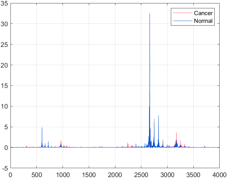
Due to the number of eigenvalues of a $n$-order matrix is $n$ (including repeated ones), we should select the samples with high dimensions to get a covariance matrix which has a large shape, and thereby obtain sufficient eigenvalue points, to observe whose relatively obvious pattern. Therefore, I decided to choose ovariancancer.mat data set, which totally contains $216$ observations (signals), including $121$ Cancer samples and $95$ Normal samples:
1
2
3
4
5
6
7
8
9
10
11
12
13
14
15
16
17
18
19
clc,clear,close all

load ovariancancer.mat

classes = unique(grp);
celldisp(classes)

obs_cancer = obs(strcmp(grp,classes{1}),:);
obs_normal = obs(strcmp(grp,classes{2}),:);
disp(height(obs_cancer))
disp(height(obs_normal))

figure
hold(gca,"on"),box(gca,"on"),grid(gca,"on")
plot(obs_cancer(1,:),"DisplayName","Cancer",...
    "Color",[249,82,107]/255,"LineWidth",0.5)
plot(obs_normal(1,:),"DisplayName","Normal",...
    "Color",[7,84,213]/255,"LineWidth",0.5)
legend();
1
2
3
4
5
6
7
8
classes{1} =
Cancer

classes{2} =
Normal

   121
    95

and each sample has $4,000$ data points.
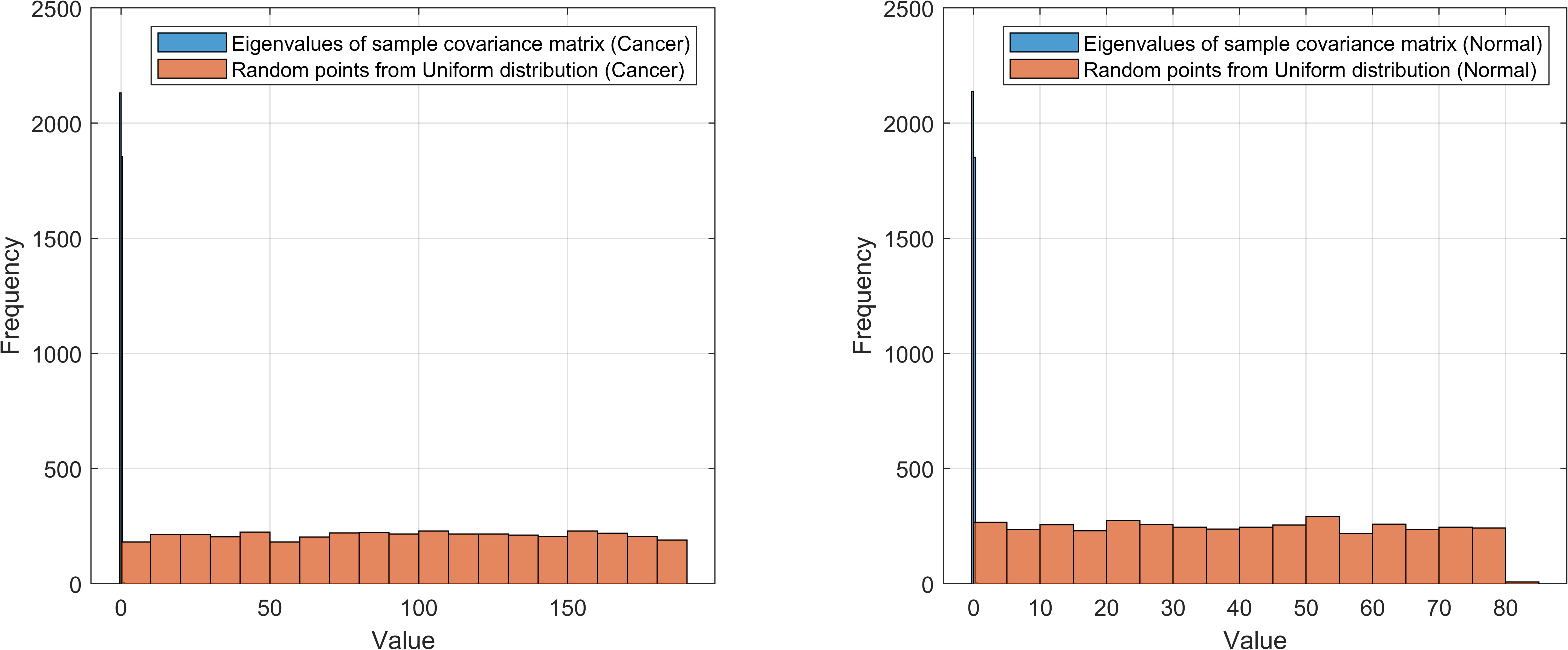
Afterwards, I plotted the distributions of sample covariance matrix eigenvalues and uniform-distributed random points among the same range for both classes:
1
2
3
4
5
6
7
8
9
10
11
12
13
14
15
16
17
18
19
20
21
22
23
24
25
26
27
28
29
30
31
32
33
34
35
36
37
38
39
40
41
42
43
44
45
46
47
48
49
50
51
52
53
54
55
56
clc,clear,close all

load ovariancancer.mat
rng("default")

classes = unique(grp);

obs_cancer = obs(strcmp(grp,classes{1}),:);
obs_normal = obs(strcmp(grp,classes{2}),:);

[cov_cancer,eigValues_cancer,uniRandomPoints_cancer] = helperFcn(obs_cancer);
[cov_normal,eigValues_normal,uniRandomPoints_normal] = helperFcn(obs_normal);

figure("Units","pixels","Position",[71,482.33,2399.33,253.99])
hold(gca,"on"),box(gca,"on"),grid(gca,"on")
markerSize = 15;
alpha = 0.7;
scatter(eigValues_cancer,1*ones(1,numel(eigValues_cancer)),markerSize, ...
    "filled","DisplayName","Eigenvalues of sample covariance matrix (Cancer)","MarkerFaceAlpha",alpha)
scatter(uniRandomPoints_cancer,2*ones(1,numel(uniRandomPoints_cancer)),markerSize, ...
    "filled","DisplayName","Random points from Uniform distribution (Cancer)","MarkerFaceAlpha",alpha)
scatter(eigValues_normal,3*ones(1,numel(eigValues_normal)),markerSize, ...
    "filled","DisplayName","Eigenvalues of sample covariance matrix (Normal)","MarkerFaceAlpha",alpha)
scatter(uniRandomPoints_normal,4*ones(1,numel(uniRandomPoints_normal)),markerSize, ...
    "filled","DisplayName","Random points from Uniform distribution (Normal)","MarkerFaceAlpha",alpha)
legend("Location","northoutside","Orientation","horizontal","FontSize",11)
set(gca,"yticklabel",[])
xlabel("Value")
exportgraphics(gcf,"pic-1.jpg","Resolution",600)

figure("Position",[483,325,1101,420])
tiledlayout(1,2)
nexttile
hold(gca,"on"),box(gca,"on"),grid(gca,"on")
histogram(eigValues_cancer,"FaceAlpha",alpha,"DisplayName","Eigenvalues of sample covariance matrix (Cancer)")
histogram(uniRandomPoints_cancer,"FaceAlpha",alpha,"DisplayName","Random points from Uniform distribution (Cancer)")
xlabel("Value")
ylabel("Frequency")
legend()
nexttile
hold(gca,"on"),box(gca,"on"),grid(gca,"on")
histogram(eigValues_normal,"FaceAlpha",alpha,"DisplayName","Eigenvalues of sample covariance matrix (Normal)")
histogram(uniRandomPoints_normal,"FaceAlpha",alpha,"DisplayName","Random points from Uniform distribution (Normal)")
xlabel("Value")
ylabel("Frequency")
legend()
exportgraphics(gcf,"pic-2.jpg","Resolution",600)

function [sampleMeanMatrix,eigValues,uniRandomPoints] = helperFcn(features)
% Calculate sample mean matrix and whose eigenvalues
sampleMeanMatrix = cov(features);
eigValues = eig(sampleMeanMatrix);

% Random ponits drawn from uniform distribution,
uniRandomPoints = sort(rand(1,height(sampleMeanMatrix))*(max(eigValues)-min(eigValues))+min(eigValues));
end


As can be seen, most eigenvalues of sample covariance matrix are very small, and the maximum eigenvalue is relatively large:
1
2
3
4
5
>> sum(eigValues_cancer<0.001),sum(eigValues_normal<0.001)
ans =
        3880
ans =
        3906
1
2
3
4
5
6
7
>> max(eigValues_cancer),max(eigValues_normal)
ans =
  single
  188.8327
ans =
  single
   80.2242
This is very different from the distributions of eigenvalues of random Hermitian matrix1.
I speculate it could be partly attributed to the large condition number of sample covariance matrix:
1
2
3
4
5
6
7
8
>> cond(cov_cancer),cond(cov_normal)
ans =
  single
  7.5149e+14

ans =
  single
  2.5022e+14
i.e., these two sample covariance matrix is ill-conditioned.
The definition of conditional number $\text{Cond}(A)$ is:
\[\begin{split} \text{Cond}(A)=&\vert\vert A\vert\vert\cdot\vert\vert A^{-1}\vert\vert\\ =&\sqrt{\max(\text{eig}(A^TA))}\cdot\sqrt{\max(\text{eig}((A^{-1})^TA^{-1}))}\\ \end{split}\label{eq1}\]I think $\text{Cond}(A)$ could imply a large $\max(\text{eig}(A))$ in a way, although $\text{Cond}(A)$ does not directly relate to $\max(\text{eig}(A))$ according to formula $\eqref{eq1}$.
References