Mardia’s test (A Multivariate Normality Test)

Oct. 23, 2023

IntroductionPermalink

Mardia’s test is a multivariate normally test to examine a set of data whether follow a multivariate normal distribution, by means of checking whether the multivariate skewness and kurtosis measures are consistent with a multivariate normal distribution [1]. The null hypothesis of Mardia’s test is that the data set is similar to the multivariate normal distribution, therefore a sufficiently small $p$ -value indicates non-normal data [2]. In addition, Mardia’s tests are affine invariant but not consistent. For example, the multivariate skewness test is NOT consistent against symmetric non-normal alternatives [2].

Recently, I found three resources on the Internet discussing Mardia’s test. The null hypothesis of them is the same, but the test statistics are not exactly the same. So, this blog will discuss about them and then make a comparison.

Mardia’s test obtained from Wikipedia [2] Permalink

For samples $X_{1}, X_{2}, \dots, X_{n}$ of $k$ -dimensional vectors, let $\hat{Σ}$ and element $m_{i, j}$ respectively denote:

\begin{matrix} (1) & \begin{aligned} \hat{Σ} = \frac{1}{n} \sum_{j = 1}^{n} (X_{j} - \bar{X}) (X_{j} - \bar{X})^{T} \\ m_{i, j} = (X_{i} - \bar{X})^{T} {\hat{Σ}}^{- 1} (X_{j} - \bar{X}) \end{aligned} \end{matrix}

N.B., Actually, $\hat{Σ}$ is the biased sample covariance matrix.

and then, we could construct test statistic $A$ and $B$ [1]:

\begin{matrix} (2) & \begin{aligned} A = \frac{1}{6 n} \sum_{i = 1}^{n} \sum_{j = 1}^{n} m_{i, j}^{3} \\ B = \sqrt{\frac{n}{8 k (k + 2)}} {\frac{1}{n} \sum_{i = 1}^{n} m_{i, i}^{2} - k (k + 2)} \end{aligned} \end{matrix}

Under the null hypothesis of multivariate normality, the statistic $A$ will have approximately a chi-squared distribution with $\frac{1}{6} k (k + 1) (k + 2)$ degrees of freedom, and $B$ will be approximately standard normal distribution $N (0, 1)$ , that is:

\begin{matrix} (3) & \begin{aligned} \frac{1}{6 n} \sum_{i = 1}^{n} \sum_{j = 1}^{n} m_{i, j}^{3} \sim χ^{2} (\frac{k (k + 1) (k + 2)}{6}) \\ \sqrt{\frac{n}{8 k (k + 2)}} {\frac{1}{n} \sum_{i = 1}^{n} m_{i, i}^{2} - k (k + 2)} \sim N (0, 1) \end{aligned} \end{matrix}

Mardia’s test obtained from “Real Statistics Using Excel” [1] Permalink

In the Mardia’s test described in “Real Statistics Using Excel” website, the test statistics are [1]:

\begin{matrix} (4) & \begin{aligned} skew = \frac{1}{n^{2}} \sum_{i = 1}^{n} \sum_{j = 1}^{n} m_{i, j}^{3} \\ kurt = \frac{1}{n} \sum_{i = 1}^{n} m_{i, i}^{2} \end{aligned} \end{matrix}

and the “sample versions” of them are:

\begin{matrix} (5) & \begin{aligned} {skew}^{'} = \frac{n}{(n - 1)^{3}} \sum_{i = 1}^{n} \sum_{j = 1}^{n} m_{i, j}^{3} \\ {kurt}^{'} = \frac{n}{(n - 1)^{2}} \sum_{i = 1}^{n} m_{i, i}^{2} \end{aligned} \end{matrix}

In addition, for small samples (generally sample size is less than 20), they could be corrected to:

\begin{matrix} (6) & \begin{aligned} {skew}^{''} & = \frac{n^{2} c}{6 (n - 1)^{3}} \sum_{i = 1}^{n} \sum_{j = 1}^{n} m_{i, j}^{3} \\ {kurt}^{''} & = \sqrt{\frac{n}{8 k (k + 2)}} [\frac{n}{(n - 1)^{2}} \sum_{i = 1}^{n} m_{i, i}^{2} - k (k + 2)] \end{aligned} \end{matrix}

where $c$ in ${skew}^{''}$ is:

\begin{matrix} (7) & c = \frac{(n + 1) (n + 3) (k + 1)}{n (n + 1) (k + 1) - 6} \end{matrix}

If accepting null hypothesis, we have:

\begin{matrix} (8) & \begin{aligned} {skew}^{''} \sim χ^{2} (\frac{k (k + 1) (k + 2)}{6}) \\ {kurt}^{''} \sim N (0, 1) \end{aligned} \end{matrix}

that is:

\begin{matrix} (9) & \begin{aligned} \frac{n^{2} c}{6 (n - 1)^{3}} \sum_{i = 1}^{n} \sum_{j = 1}^{n} m_{i, j}^{3} \sim χ^{2} (\frac{k (k + 1) (k + 2)}{6}) \\ \sqrt{\frac{n}{8 k (k + 2)}} [\frac{n}{(n - 1)^{2}} \sum_{i = 1}^{n} m_{i, i}^{2} - k (k + 2)] \sim N (0, 1) \end{aligned} \end{matrix}

The red marks in above equation represents the coefficients that are different from equation $(3)$ . As can be seen, if $n \to \infty$ , equation $(9)$ is the same as $(3)$ , so these could be viewed as some corrections in small sample case. I don’t make a profound study for these coefficients, but I feel $n - 1$ is from the correction for high sample moments, something like Bessel’s correction [4, 5, 6].

Mardia’s test obtained from MATLAB official example [3] Permalink

MATLAB documentation also provides an example to illustrate how to perform Mardia Kurtosis Test from Linear and Quadratic discriminant models [3] (both model are constructed using fitcdiscr function, some concerned content about this function could be found in blog [7] and official documentation [8]), and the test for linear model is like:

matlab

load fisheriris;
prednames = {'SepalLength','SepalWidth','PetalLength','PetalWidth'};

% Train a linear discriminant analysis model.
L = fitcdiscr(meas,species,'PredictorNames',prednames);

[N,D] = size(meas);

meanL = mean(mahal(L,L.X,'ClassLabels',L.Y).^2);
[~,pvalL] = ztest(meanL,D*(D+2),sqrt(8*D*(D+2)/N))

As can be seen:

(1) This test is just examine kurtosis, without skew.

(2) The $z$ -test is used to test kurtosis, and the null hypothesis of it is:

\begin{matrix} (10) & \frac{1}{n} \sum_{i = 1}^{n} m_{i, i}^{2} \sim N (k (k + 2), \sqrt{\frac{8 k (k + 2)}{n}}) \end{matrix}

i.e.,

\begin{matrix} (11) & (\frac{n}{8 k (k + 2)})^{1 / 4} [\frac{1}{n} \sum_{i = 1}^{n} m_{i, i}^{2} - k (k + 2)] \sim N (0, 1) \end{matrix}

It is like Mardia’s test provided by Wikipedia (equation $(3)$ ), but the coefficient is $(\frac{n}{8 k (k + 2)})^{1 / 4}$ rather than $(\frac{n}{8 k (k + 2)})^{1 / 2}$ . I tend to contend that the MATLAB example made a mistake at this aspect.

(3) This example calculates $(1 / n) \sum_{i = 1}^{n} m_{i, i}^{2}$ by calculating (squared) Mahalanobis distance using mahal function (could refer to blog [9]):

matlab

meanL = mean(mahal(L,L.X,'ClassLabels',L.Y).^2);

It is convenient, but the results it is kind of different from those results based on equations $(1)$ , as $\hat{Σ}$ in equation $(1)$ is biased sample covariance matrix, but mahal function calculate based on unbiased sample covariance matrix. We could simply make a verification:

matlab

clc,clear,close all

load fisheriris.mat
meas = meas(1:50,:);

[n,k] = size(meas);
mu = mean(meas);

% Calculate the sum of m_ii by matrix multiplication (biased)
Sigma_biased = cov(meas,1); % biased SCM
b_biased = ((meas-mu)/Sigma_biased*(meas-mu)').^2;
b_biased = sum(b_biased.*diag(ones(1,height(b_biased))),"all")/n;

% Calculate the sum of m_ii by matrix multiplication (unbiased)
Sigma_unbiased = cov(meas,0); % deffault setting: 0, unbiased SCM
b_unbiased = ((meas-mu)/Sigma_unbiased*(meas-mu)').^2;
b_unbiased = sum(b_unbiased.*diag(ones(1,height(b_unbiased))),"all")/n;

% Calculate the sum of m_ii by `mahal` function
b_mahal= mean(mahal(meas,meas).^2);

fprintf("Calculate the sum of m_ii by matrix multiplication (biased): %.4f,\n" + ...
    "Calculate the sum of m_ii by matrix multiplication (unbiased): %.4f,\n" + ...
    "Calculate the sum of m_ii by `mahal` function: %.4f.\n", ...
    b_biased,b_unbiased,b_mahal)

plaintext

Calculate the sum of m_ii by matrix multiplication (biased): 26.5377,
Calculate the sum of m_ii by matrix multiplication (unbiased): 25.4868,
Calculate the sum of m_ii by `mahal` function: 25.4868.

On another hand, MATLAB mahal doesn’t adopt an obvious way to calculate $(1 / n) \sum_{i = 1}^{n} m_{i, i}^{2}$ by directly calculating and then inversing $\hat{Σ}$ , but relies on orthogonal-triangular decomposition:

Maybe it is a more robust numerical computation method, but I don’t understand it right now, so in the following text, I still use matrix multiplication to be consistent with $(1)$ .

Compared experimentsPermalink

Experiment 1: preliminary compared experimentPermalink

As described above, the Mardia’s test from MATLAB example is not complete (as it does not test skewness), and the coefficient is not appropriate. So, I would contrast the first two calculation method in this part, i.e., the formula provided by Wikipedia $(3)$ and that provided by “Real Statistics Using Excel” $(9)$ .

To compare two methods, I hope the samples which to be tested actually from a multivariate normal distribution, i.e., generated by MATLAB mvnrnd function. However, the parameter Simga passed into mvnrnd must be positive semi-definite matrix. This is kind of strict, and should be carefully designed. But luckily, we could prove that the sample covariance matrix is ALWAYS positive semi-definite (see [10]). So, I choose the features of “setosa” class from fisheriris data set, and use moments estimation method to estimate $\hat{μ}$ and $\hat{Σ}$ of them, and based on which generate a certain amount of samples using mvnrnd, whose sample size is $20$ , $50$ , $100$ , $500$ , $1, 000$ , $10, 000$ , or $20, 000$ respectively; the following verifications are conducted on these generated samples. In addition, I mainly make analysis based on the the $p$ -value of each test.

matlab

clc,clear,close all

rng(1)

load fisheriris.mat
meas = meas(1:50,:);

mu = mean(meas);
Sigma = cov(meas);
numGs = [20,50,100,500,1000,1e4,2e4];

pValue_As = nan(1,numel(numGs));
pValue_Bs = nan(1,numel(numGs));
pValue_skew_correcteds = nan(1,numel(numGs));
pValue_kurt_correcteds = nan(1,numel(numGs));

for i = 1:numel(numGs)
    [pValue_As(i),pValue_Bs(i),pValue_skew_correcteds(i),pValue_kurt_correcteds(i)] = helperMardia(mu,Sigma,numGs(i));
end

figure("Position",[197,271,1553,420])
tiledlayout(1,2)
nexttile
hold(gca,"on"),box(gca,"on"),grid(gca,"on")
stem((1:numel(numGs))-0.1,pValue_As,"LineWidth",1.5,"DisplayName","Wiki version","Color","b")
stem((1:numel(numGs))+0.1,pValue_skew_correcteds,"LineWidth",1.5,"DisplayName","Real Statistics Version","Color","r")
xticklabels(numGs)
xticks(1:numel(numGs))
xlabel("Sample size")
ylabel("p-value")
legend("Location","southeast")

nexttile
hold(gca,"on"),box(gca,"on"),grid(gca,"on")
stem((1:numel(numGs))-0.1,pValue_Bs,"LineWidth",1.5,"DisplayName","Wiki version","Color","b")
stem((1:numel(numGs))+0.1,pValue_kurt_correcteds,"LineWidth",1.5,"DisplayName","Real Statistics Version","Color","r")
xticklabels(numGs)
xticks(1:numel(numGs))
xlabel("Sample size")
ylabel("p-value")
legend("Location","southeast")

function [pValue_A,pValue_B,pValue_skew_corrected,pValue_kurt_corrected] = helperMardia(mu,Sigma,numG)
% Generate samples
data = mvnrnd(mu,Sigma,numG);

[n,k] = size(data);
Sigma_hat = cov(data,0); % biased SCM
a = sum(((data-mu)/Sigma_hat*(data-mu)').^3,"all");
b = ((data-mu)/Sigma_hat*(data-mu)').^2;
b = sum(b.*diag(ones(1,height(b))),"all");

df = (1/6)*k*(k+1)*(k+2);

% % Wikipedia version Mardia's test
A = (1/6/n)*a;
B = sqrt(n/(8*k*(k+2)))*(1/n*b-k*(k+2));
pValue_A = chi2cdf(A,df);
[~,pValue_B,~,~] = ztest(B,0,1);
% pValue_B = 2*normcdf(B,0,1)

% % Real Statistics version Mardia's test
c = (n+1)*(n+3)*(k+1)/(n*(n+1)*(k+1)-6);
skew_corrected = (n^2)*c/(6*(n-1)^3)*a;
kurt_corrected = sqrt(n/(8*k*(k+2)))*(n/((n-1)^2)*b-k*(k+2));
pValue_skew_corrected = chi2cdf(skew_corrected,df);
[~,pValue_kurt_corrected,~,~] = ztest(kurt_corrected,0,1);
% pValue_kurt_corrected = 2*normcdf(kurt_corrected,0,1)

% fprintf("Wikipedia version Mardia's test\n" + ...
%     "p-value of the test for A: %.4f,\np-value of the test for B: %.4f\n" + ...
%     "Real Statistics version Mardia's test\n" + ...
%     "p-value of the test for skewness: %.4f,\np-value of the test for kurtosis: %.4f\n", ...
%     pValue_A,pValue_B,pValue_skew_corrected,pValue_kurt_corrected);
end

The results show that, as was expected, no matter which formula is adopted, we could accept the null hypothesis anyway, and as sample size increases, both test results approached asymptotically. However, the sample size actually influence our confidence. What’s more, when sample size is small, there exist a difference between two test results, and this difference is irregular in this experiment.

Experiment 2: try more different sample sizesPermalink

If we try more different sample sizes to see a more detail result:

matlab

clc,clear,close all

rng(1)

load fisheriris.mat
meas = meas(1:50,:);

mu = mean(meas);
Sigma = cov(meas);
numGs = 10:10:1000;
% numGs = 1e3:100:1e4;
% numGs = 1e4:200:2e4;

pValue_As = nan(1,numel(numGs));
pValue_Bs = nan(1,numel(numGs));
pValue_skew_correcteds = nan(1,numel(numGs));
pValue_kurt_correcteds = nan(1,numel(numGs));

for i = 1:numel(numGs)
    [pValue_As(i),pValue_Bs(i),pValue_skew_correcteds(i),pValue_kurt_correcteds(i)] = helperMardia(mu,Sigma,numGs(i));
end

figure("Position",[197,30,1553,840],"Color","w")
tiledlayout(2,1)
nexttile
hold(gca,"on"),box(gca,"on"),grid(gca,"on")
plot(numGs,pValue_As,"LineWidth",1.5,"DisplayName","Wiki version","Color","b","Marker","o")
plot(numGs,pValue_skew_correcteds,"LineWidth",1.5,"DisplayName","Real Statistics Version","Color","r","Marker","square")
% xticklabels(numGs)
% xticks(1:numel(numGs))
xlabel("Sample size")
ylabel("p-value")
legend("Location","southeast")
title("Test for skewness")
ylim([0,1])

nexttile
hold(gca,"on"),box(gca,"on"),grid(gca,"on")
plot(numGs,pValue_Bs,"LineWidth",1.5,"DisplayName","Wiki version","Color","b","Marker","o")
plot(numGs,pValue_kurt_correcteds,"LineWidth",1.5,"DisplayName","Real Statistics Version","Color","r","Marker","square")
% xticklabels(numGs)
% xticks(1:numel(numGs))
xlabel("Sample size")
ylabel("p-value")
legend("Location","southeast")
title("Test for kurtosis")
ylim([0,1])

function [pValue_A,pValue_B,pValue_skew_corrected,pValue_kurt_corrected] = helperMardia(mu,Sigma,numG)
% Generate samples
data = mvnrnd(mu,Sigma,numG);

[n,k] = size(data);
Sigma_hat = cov(data,0); % biased SCM
a = sum(((data-mu)/Sigma_hat*(data-mu)').^3,"all");
b = ((data-mu)/Sigma_hat*(data-mu)').^2;
b = sum(b.*diag(ones(1,height(b))),"all");

df = (1/6)*k*(k+1)*(k+2);

% % Wikipedia version Mardia's test
A = (1/6/n)*a;
B = sqrt(n/(8*k*(k+2)))*(1/n*b-k*(k+2));
pValue_A = chi2cdf(A,df);
[~,pValue_B,~,~] = ztest(B,0,1);
% pValue_B = 2*normcdf(B,0,1)

% % Real Statistics version Mardia's test
c = (n+1)*(n+3)*(k+1)/(n*(n+1)*(k+1)-6);
skew_corrected = (n^2)*c/(6*(n-1)^3)*a;
kurt_corrected = sqrt(n/(8*k*(k+2)))*(n/((n-1)^2)*b-k*(k+2));
pValue_skew_corrected = chi2cdf(skew_corrected,df);
[~,pValue_kurt_corrected,~,~] = ztest(kurt_corrected,0,1);
% pValue_kurt_corrected = 2*normcdf(kurt_corrected,0,1)

% fprintf("Wikipedia version Mardia's test\n" + ...
%     "p-value of the test for A: %.4f,\np-value of the test for B: %.4f\n" + ...
%     "Real Statistics version Mardia's test\n" + ...
%     "p-value of the test for skewness: %.4f,\np-value of the test for kurtosis: %.4f\n", ...
%     pValue_A,pValue_B,pValue_skew_corrected,pValue_kurt_corrected);
end

results-Epoch1-1000

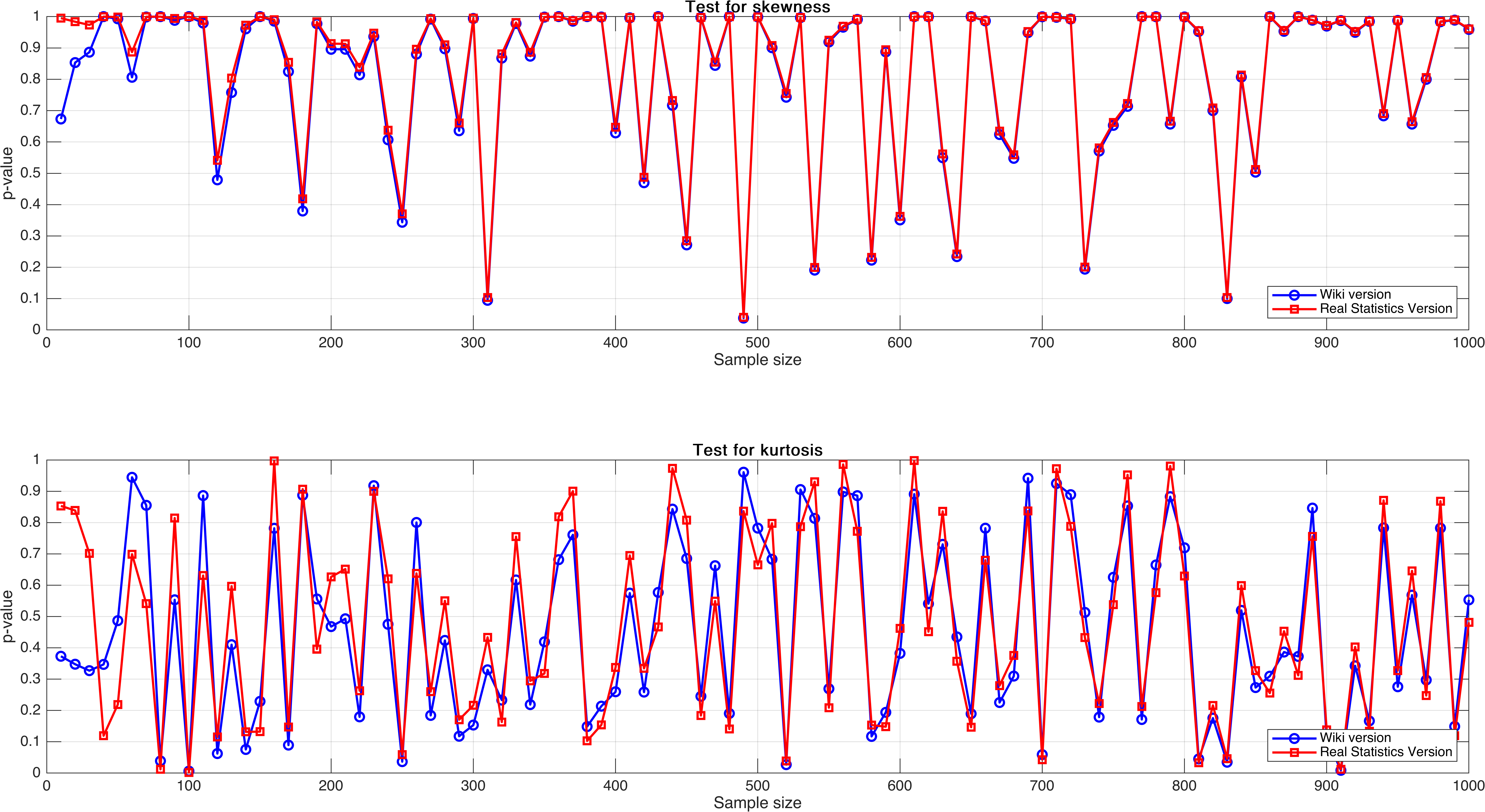
Sample size varies from $10$ to $1, 000$ , with step $10$ .

results-Epoch1-10000

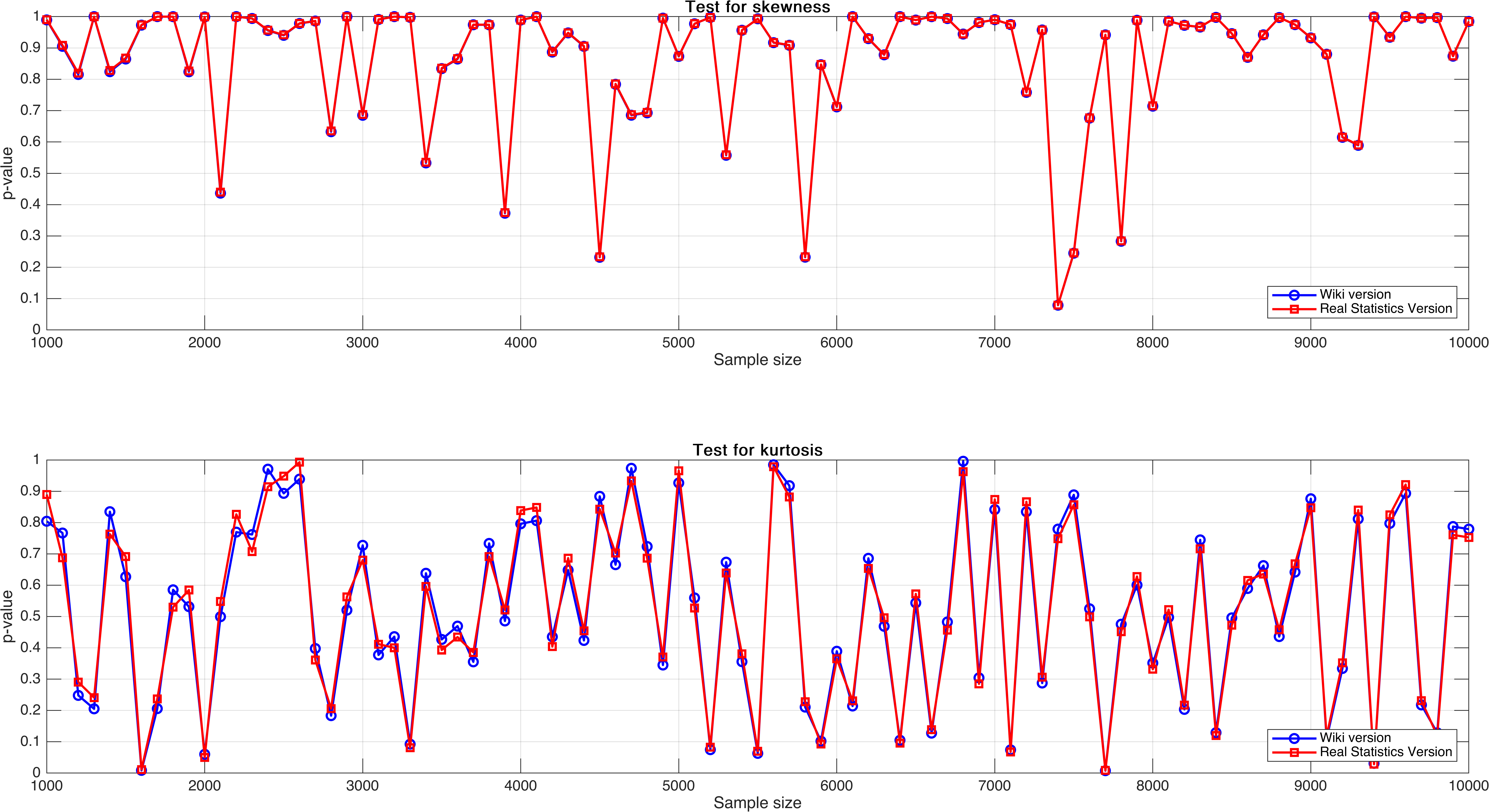
Sample size varies from $1, 000$ to $10, 000$ , with step $100$ .

results-Epoch1-20000

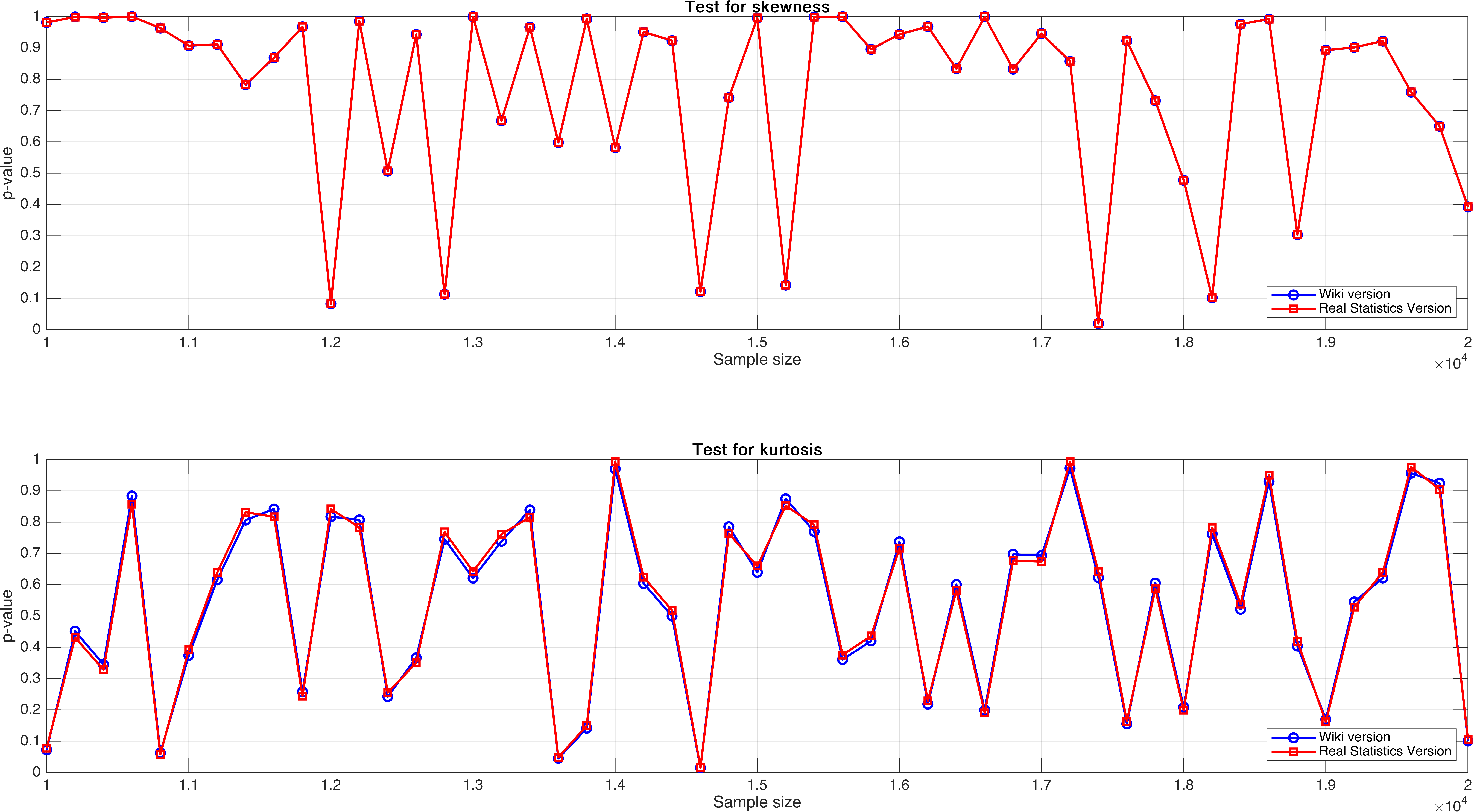
Sample size varies from $10, 000$ to $20, 000$ , with step $200$ .

In this experiment, I expect to see a regular pattern, for example, there exist a relatively obvious increasing trend as sample size increases, but unluckily, it doesn’t, and what’s worse is that the $p$ -value seemingly not stable.

Experiment 3: observe mean $p$ -valuesPermalink

So, I continue to experiment. This set of experiments is analogous with Experiment 2. The difference is that, in this part, every Mardia’s test is repeatedly conducted multiple times under the same sample size, and therefore the figures show mean $p$ -value.

matlab

clc,clear,close all

rng(1)

load fisheriris.mat
meas = meas(1:50,:);

mu = mean(meas);
Sigma = cov(meas);

numEpoch = 20;

numGs = 10:10:1000;
% numGs = 1e3:100:1e4;
% numGs = 1e4:200:2e4;

pValue_As = nan(1,numel(numGs));
pValue_Bs = nan(1,numel(numGs));
pValue_skew_correcteds = nan(1,numel(numGs));
pValue_kurt_correcteds = nan(1,numel(numGs));

for j = 1:numEpoch
    disp(j)
    for i = 1:numel(numGs)
        [pValue_As(j,i),pValue_Bs(j,i),pValue_skew_correcteds(j,i),pValue_kurt_correcteds(j,i)] = helperMardia(mu,Sigma,numGs(i));
    end
end

save("results.mat","pValue_As","pValue_Bs","pValue_skew_correcteds","pValue_kurt_correcteds")
pValue_As = mean(pValue_As,1);
pValue_Bs = mean(pValue_Bs,1);
pValue_skew_correcteds = mean(pValue_skew_correcteds,1);
pValue_kurt_correcteds = mean(pValue_kurt_correcteds,1);

figure("Position",[197,30,1553,840],"Color","w")
tiledlayout(2,1)
nexttile
hold(gca,"on"),box(gca,"on"),grid(gca,"on")
plot(numGs,pValue_As,"LineWidth",1.5,"DisplayName","Wiki version","Color","b","Marker","o")
plot(numGs,pValue_skew_correcteds,"LineWidth",1.5,"DisplayName","Real Statistics Version","Color","r","Marker","square")
xlabel("Sample size")
ylabel("p-value")
legend("Location","southeast")
title(sprintf("Test for skewness (the number of repeated experiment: %s)",num2str(numEpoch)))
ylim([0,1])

nexttile
hold(gca,"on"),box(gca,"on"),grid(gca,"on")
plot(numGs,pValue_Bs,"LineWidth",1.5,"DisplayName","Wiki version","Color","b","Marker","o")
plot(numGs,pValue_kurt_correcteds,"LineWidth",1.5,"DisplayName","Real Statistics Version","Color","r","Marker","square")
xlabel("Sample size")
ylabel("p-value")
legend("Location","southeast")
title(sprintf("Test for kurtosis (the number of repeated experiment: %s)",num2str(numEpoch)))
ylim([0,1])

pngFileName = sprintf("results-Epochs%s-%s.png",num2str(numEpoch),num2str(numGs(end)));
exportgraphics(gcf,pngFileName,"Resolution",600)
matFileName = sprintf("results-Epochs%s-%s.mat",num2str(numEpoch),num2str(numGs(end)));
save(matFileName,"pValue_As","pValue_Bs","pValue_skew_correcteds","pValue_kurt_correcteds")

function [pValue_A,pValue_B,pValue_skew_corrected,pValue_kurt_corrected] = helperMardia(mu,Sigma,numG)
% Generate samples
data = mvnrnd(mu,Sigma,numG);

[n,k] = size(data);
Sigma_hat = cov(data,0); % biased SCM
a = sum(((data-mu)/Sigma_hat*(data-mu)').^3,"all");
b = ((data-mu)/Sigma_hat*(data-mu)').^2;
b = sum(b.*diag(ones(1,height(b))),"all");

df = (1/6)*k*(k+1)*(k+2);

% % Wikipedia version Mardia's test
A = (1/6/n)*a;
B = sqrt(n/(8*k*(k+2)))*(1/n*b-k*(k+2));
pValue_A = chi2cdf(A,df);
[~,pValue_B,~,~] = ztest(B,0,1);
% pValue_B = 2*normcdf(B,0,1)

% % Real Statistics version Mardia's test
c = (n+1)*(n+3)*(k+1)/(n*(n+1)*(k+1)-6);
skew_corrected = (n^2)*c/(6*(n-1)^3)*a;
kurt_corrected = sqrt(n/(8*k*(k+2)))*(n/((n-1)^2)*b-k*(k+2));
pValue_skew_corrected = chi2cdf(skew_corrected,df);
[~,pValue_kurt_corrected,~,~] = ztest(kurt_corrected,0,1);
% pValue_kurt_corrected = 2*normcdf(kurt_corrected,0,1)

% fprintf("Wikipedia version Mardia's test\n" + ...
%     "p-value of the test for A: %.4f,\np-value of the test for B: %.4f\n" + ...
%     "Real Statistics version Mardia's test\n" + ...
%     "p-value of the test for skewness: %.4f,\np-value of the test for kurtosis: %.4f\n", ...
%     pValue_A,pValue_B,pValue_skew_corrected,pValue_kurt_corrected);
end

results-Epochs20-1000

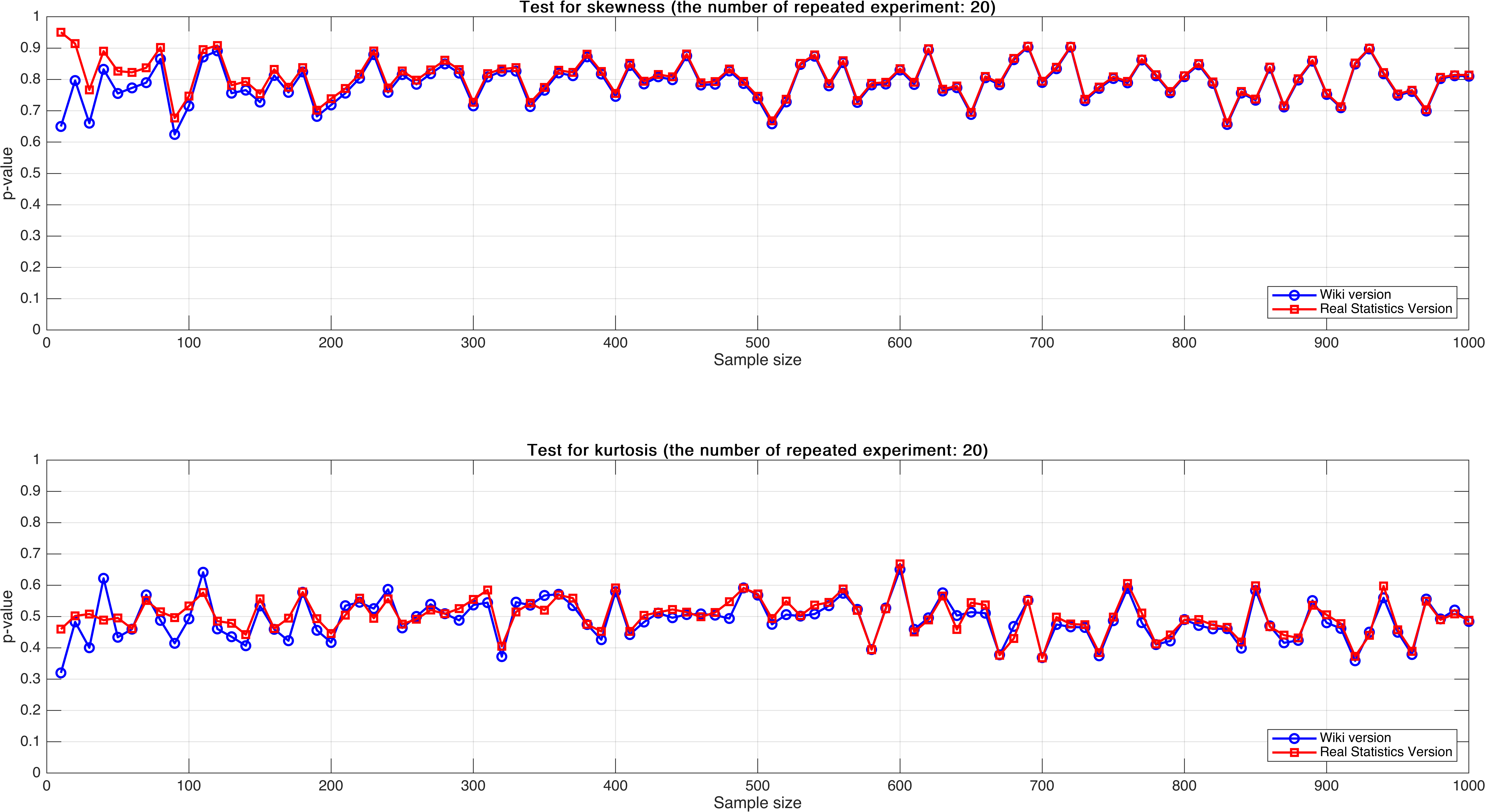
Sample size varies from $10$ to $1, 000$ , with step $10$ , mean $p$ -value of $20$ times.

results-Epochs20-10000

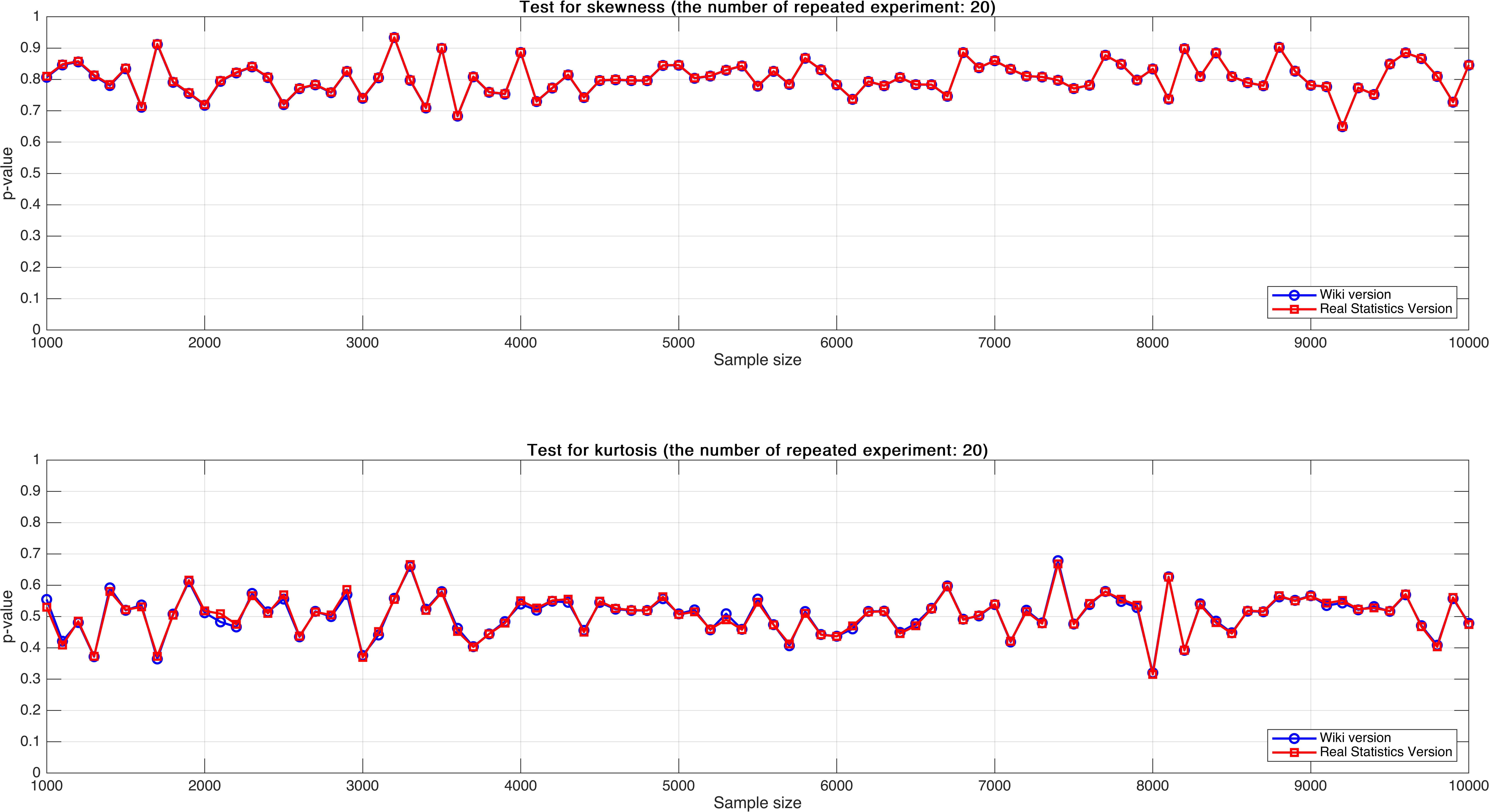
Sample size varies from $1, 000$ to $10, 000$ , with step $100$ , mean $p$ -value of $20$ times.

results-Epochs20-20000

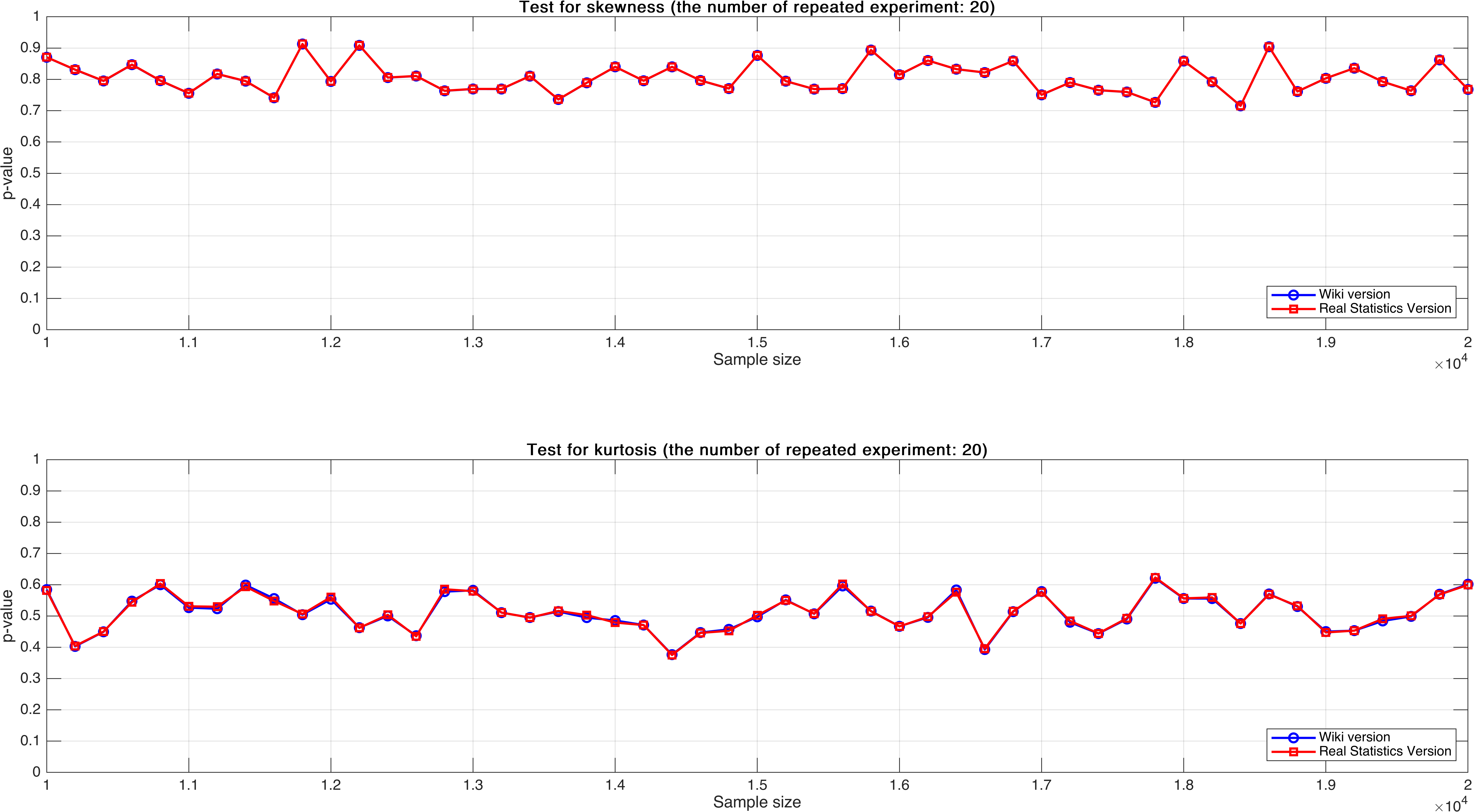
Sample size varies from $10, 000$ to $20, 000$ , with step $200$ , mean $p$ -value of $20$ times.

As can be seen, the mean $p$ -value seems more stable than $p$ -value of single test that in Experiment 2.

If we increase the number of repeated experiment from $20$ times to $10, 000$ times, we could get:

results-Epochs10000-1000

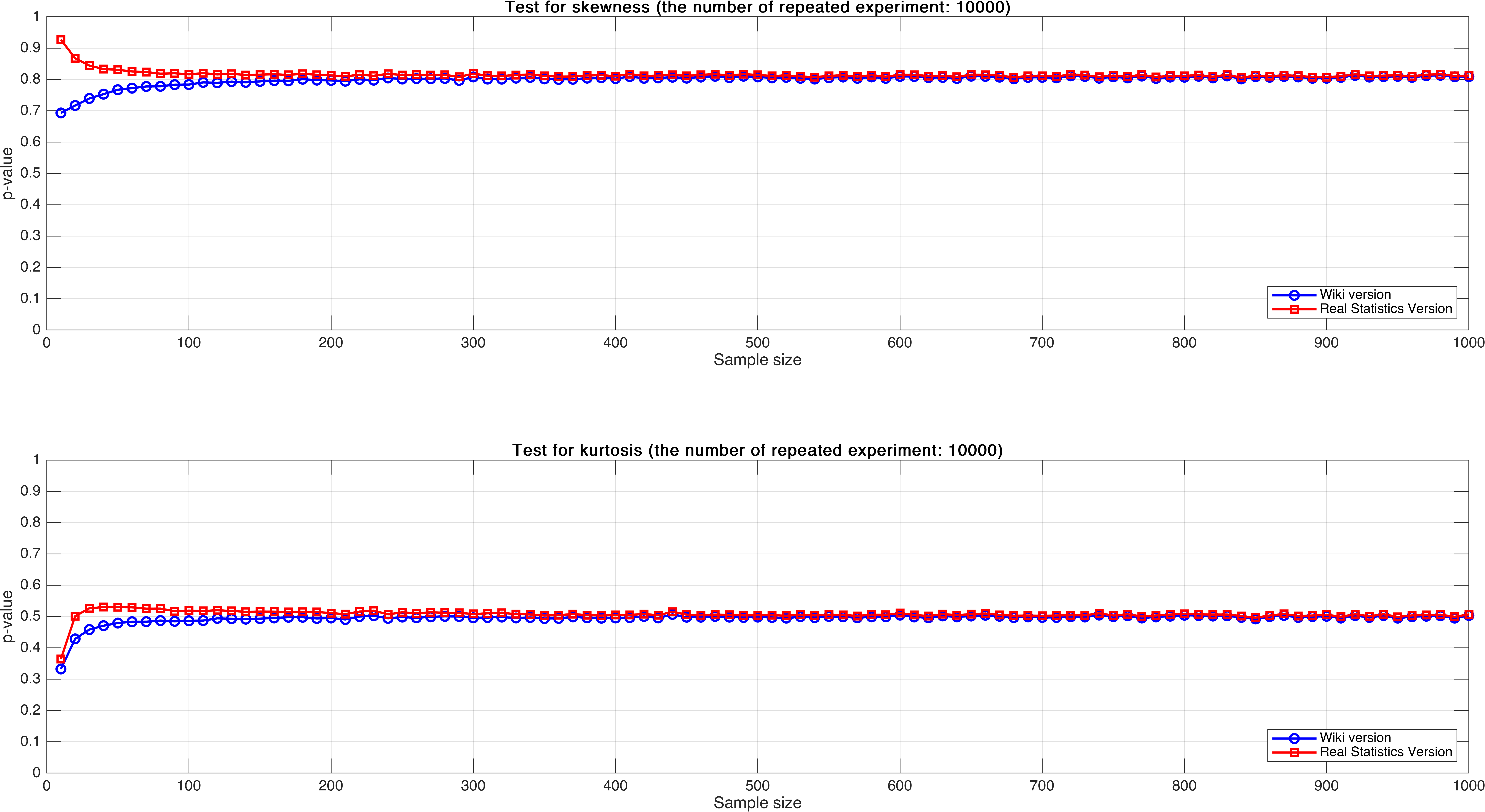
Sample size varies from $10$ to $1, 000$ , with step $10$ , mean $p$ -value of $10, 000$ times.

At this time, we could see obvious patterns:

For both “Test for skewness”and “Test for kurtosis”, the results of $(3)$ and $(9)$ are stable and consistent as sample size increases, especially when sample size is over $300$ .
For both “Test for skewness”and “Test for kurtosis”, when sample size is relatively small, we have more confidence to accept null hypothesis according to $(9)$ compared with $(3)$ . This is brought by correction $(6)$ .
For “Test for skewness”, the $p$ -value corresponding to $(9)$ decreases as sample size increases, however, $p$ -value corresponding to $(3)$ increases. And For “Test for kurtosis”, $p$ -value corresponding to both $(3)$ and $(9)$ increases as sample size increases.

DiscussionsPermalink

From above experiments, we could see that:

The results of Mardia’s test with small sample size is not reliable;
The results of a single Mardia’s test is not reliable if samples are random, because“random number”will significantly influence our confidence.

To overcome these problems, we should collect samples as much as possible to get them involved in the Mardia’s test, and carry out repeated tests to relieve the influence of random factors.

References

[1] Mardia’s Test - Real Statistics Using Excel.

[2] Multivariate normal distribution: Multivariate normality tests - Wikipedia.

[3] Examine the Gaussian Mixture Assumption: Mardia-Kurtosis Test for Linear and Quadratic Discriminants - MathWorks.

[4] Bessel’s correction - Wikipedia.

[5] Estimation of covariance matrices - Wikipedia.

[6] From Sample Covariance Matrix(SCM) to Bessel’s Correction - What a starry night~.

[7] MATLAB fitcdiscr Function - What a starry night~.

[8] fitcdiscr: Fit discriminant analysis classifier. - MathWorks.

[9] Multivariate Normal Distribution and Mahalanobis Distance: Mahalanobis Distance - What a starry night~.

[10] Is a sample covariance matrix always symmetric and positive definite? - Stack Exchange.