MATLAB fitcdiscr Function
Note Well Here: My initial purpose of writing this blog is to explore the MATLAB fitcdiscr function. I found the official documentation describes that it is used to estimate a multivariate normal distribution, so I naturally thought it is realised by moment estimation, and therefore verified it by this way. However, in the end, I realised I was wrong (although it is a so obvious mistake when looking backward at present). The reason could be found in the last part Hyperparameter Optimizsation Options and Discussions. Having said that, I believe this is a valuable process in a way, so I decide to organise these content in this blog.
Introduction
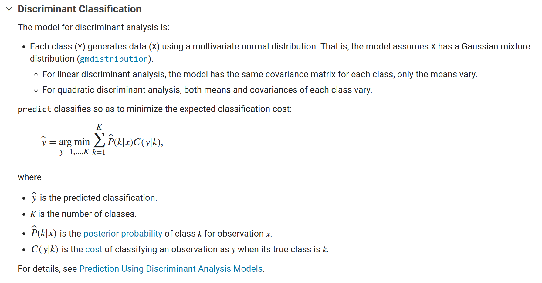
MATLAB fitcdiscr function [1] is for “Fit discriminant analysis classifier”, and the algorithm introduction in the official documentation gives more information:
Taking fisheriris dataset as an example, the following text will analyse the fitcdiscr function.
Linear discriminant analysis
For sake of easy visual analysis in the later part, we select the first three features of meas variable to analyse:
1
2
3
4
5
6
load fisheriris
meas = meas(:,1:3);

mdl = fitcdiscr(meas,species); % DiscrimType: 'linear'(fault)
mus = mdl.Mu;
Sigmas = mdl.Sigma;
1
2
3
4
5
6
7
8
mus =
    5.0060    3.4280    1.4620
    5.9360    2.7700    4.2600
    6.5880    2.9740    5.5520
Sigmas =
    0.2650    0.0927    0.1675
    0.0927    0.1154    0.0552
    0.1675    0.0552    0.1852
As described, for linear discriminant analysis, the multiviriate normal distribution of each class has its own mean value, but all the classes have a common covariance matrix.
And the the mean vector of each multiviriate normal distribution is estimated by the sample mean vector of each class, but the covariance matrix is not estimated by neither the sample covariance matrix of all the samples, nor the sample covariance matrix of each class:
1
2
3
4
5
[ClassVariables,Classes] = findgroups(species);
means = splitapply(@mean,meas,ClassVariables);
Covs = splitapply(@(x){cov(x)},meas,ClassVariables);
Covs{1},Covs{2},Covs{3}
Cov_all = cov(meas);
1
2
3
4
5
6
7
8
9
10
11
12
13
14
15
16
17
18
19
20
21
>> means,celldisp(Covs),Cov_all
means =
    5.0060    3.4280    1.4620
    5.9360    2.7700    4.2600
    6.5880    2.9740    5.5520
Covs{1} =
    0.1242    0.0992    0.0164
    0.0992    0.1437    0.0117
    0.0164    0.0117    0.0302
Covs{2} =
    0.2664    0.0852    0.1829
    0.0852    0.0985    0.0827
    0.1829    0.0827    0.2208
Covs{3} =
    0.4043    0.0938    0.3033
    0.0938    0.1040    0.0714
    0.3033    0.0714    0.3046
Cov_all =
    0.6857   -0.0424    1.2743
   -0.0424    0.1900   -0.3297
    1.2743   -0.3297    3.1163
The common covariance matrix is likely the weighted average of sample covariance matrix of each class:
1
2
3
4
5
>> Covs{1}/3+Covs{2}/3+Covs{3}/3
ans =
    0.2650    0.0927    0.1675
    0.0927    0.1154    0.0552
    0.1675    0.0552    0.1852
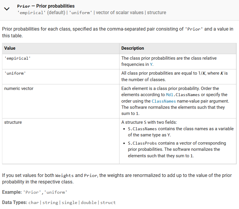
and the coefficient is seemingly determined by the mdl.Prior, which is sample number proportion of each class (default value emperical):
1
2
3
>> mdl.Prior
ans =
    0.3333    0.3333    0.3333
If we change the sample number of each class to 40, 30, and 20, respectively, and re-run the code:
>> mdl.Prior ans = 0.4444 0.3333 0.2222
>> Sigmas,mdl.Prior(1)*Covs{1}+mdl.Prior(2)*Covs{2}+mdl.Prior(3)*Covs{3} Sigmas = 0.2278 0.0976 0.1170 0.0976 0.1214 0.0501 0.1170 0.0501 0.1317 ans = 0.2285 0.0975 0.1176 0.0975 0.1212 0.0503 0.1176 0.0503 0.1323The difference between the covariance matrix of
mdland the one we calculated still exist, although small. I don’t check whether this deviation is caused by numerical calculation error.
So to my mind, strictly speaking, the description in the official documentation “the model assumes X has a Gaussian mixture distribution” is not that appropriate (at least for this case where using the default easy linear discriminant analysis), as the coefficients of GMM are not estimated but just calculated based on sample size. Another MATLAB documentation fitgmdist using EM iterative algorithm is more reasonable, the analysis of which could be found in blog [2].
After getting the sample mean and shared weighted covariance matrix, we could use mvnrnd function to generate samples, and compared them with the samples in fisheiris dataset:
1
2
3
4
5
6
7
8
9
10
11
12
13
14
15
16
17
18
19
20
21
22
23
24
25
26
27
28
29
30
31
32
33
34
35
36
37
38
39
40
41
42
43
44
45
46
47
48
49
50
51
52
53
54
55
56
clc,clear,close all

load fisheriris
meas = meas(:,1:3);

mdl = fitcdiscr(meas,species); % DiscrimType: 'linear'(fault)
mus = mdl.Mu;
Sigmas = mdl.Sigma;

numNew = 200;
newSetosa = mvnrnd(mus(1,:),Sigmas,numNew);
newVersicolor = mvnrnd(mus(2,:),Sigmas,numNew);
newVirginica = mvnrnd(mus(3,:),Sigmas,numNew);

meas_setosa = meas(strcmp(species,"setosa"),:);
meas_versicolor = meas(strcmp(species,"versicolor"),:);
meas_virginica = meas(strcmp(species,"virginica"),:);

figure("Units","pixels","Position",[390.3333333333333,465,1550,420])
tiledlayout(1,3,"TileSpacing","tight")
markerSize = 20;
nexttile
hold(gca,"on"),box(gca,"on"),grid(gca,"on"),view(3)
scatter3(meas_setosa(:,1),meas_setosa(:,2),meas_setosa(:,3), ...
    markerSize,"filled","DisplayName","Original","MarkerFaceColor",[7,84,213]/255)
scatter3(newSetosa(:,1),newSetosa(:,2),newSetosa(:,3), ...
    markerSize,"filled","DisplayName","Generated","MarkerFaceColor",[249,82,107]/255)
legend("Location","north","Orientation","horizontal");
title("Species: Setosa")
xlabel("Feature 1")
ylabel("Feature 2")
zlabel("Feature 3")

nexttile
hold(gca,"on"),box(gca,"on"),grid(gca,"on"),view(3)
scatter3(meas_versicolor(:,1),meas_versicolor(:,2),meas_versicolor(:,3), ...
    markerSize,"filled","DisplayName","Original","MarkerFaceColor",[7,84,213]/255)
scatter3(newVersicolor(:,1),newVersicolor(:,2),newVersicolor(:,3), ...
    markerSize,"filled","DisplayName","Generated","MarkerFaceColor",[249,82,107]/255)
legend("Location","north","Orientation","horizontal");
title("Species: Versicolor")
xlabel("Feature 1")
ylabel("Feature 2")
zlabel("Feature 3")

nexttile
hold(gca,"on"),box(gca,"on"),grid(gca,"on"),view(3)
scatter3(meas_virginica(:,1),meas_virginica(:,2),meas_virginica(:,3), ...
    markerSize,"filled","DisplayName","Original","MarkerFaceColor",[7,84,213]/255)
scatter3(newVirginica(:,1),newVirginica(:,2),newVirginica(:,3), ...
    markerSize,"filled","DisplayName","Generated","MarkerFaceColor",[249,82,107]/255)
legend("Location","north","Orientation","horizontal");
title("Species: Virginica")
xlabel("Feature 1")
ylabel("Feature 2")
zlabel("Feature 3")

Quadratic discriminant analysis
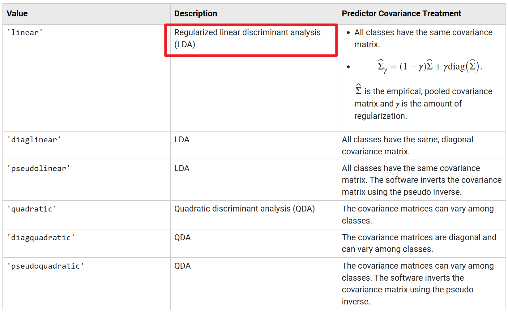
As pointed out in the official documentation [1], specifying the property DiscrimType to quadratic could make a quadratic discriminant analysis and at which case, both mean and covariance matrix of each class vary.
1
2
3
4
5
6
load fisheriris
meas = meas(:,1:3);

mdl = fitcdiscr(meas,species,"DiscrimType","quadratic"); % DiscrimType: quadratic
mus = mdl.Mu;
Sigmas = mdl.Sigma;
1
2
3
4
5
6
7
8
9
10
11
12
13
14
15
16
17
>> mus,Sigmas
mus =
    5.0060    3.4280    1.4620
    5.9360    2.7700    4.2600
    6.5880    2.9740    5.5520
Sigmas(:,:,1) =
    0.1242    0.0992    0.0164
    0.0992    0.1437    0.0117
    0.0164    0.0117    0.0302
Sigmas(:,:,2) =
    0.2664    0.0852    0.1829
    0.0852    0.0985    0.0827
    0.1829    0.0827    0.2208
Sigmas(:,:,3) =
    0.4043    0.0938    0.3033
    0.0938    0.1040    0.0714
    0.3033    0.0714    0.3046
Similarly, we could compare these parameters with the calculated ones:
1
2
3
4
5
6
7
8
9
10
11
12
13
14
15
16
17
>> means,celldisp(Covs)
means =
    5.0060    3.4280    1.4620
    5.9360    2.7700    4.2600
    6.5880    2.9740    5.5520
Covs{1} =
    0.1242    0.0992    0.0164
    0.0992    0.1437    0.0117
    0.0164    0.0117    0.0302
Covs{2} =
    0.2664    0.0852    0.1829
    0.0852    0.0985    0.0827
    0.1829    0.0827    0.2208
Covs{3} =
    0.4043    0.0938    0.3033
    0.0938    0.1040    0.0714
    0.3033    0.0714    0.3046
As can be seen, for quadratic discriminant analysis, the mean vector and covariance matrix are respectively estimated by sample mean vector and unbiased sample variance matrix of each class, that is making a unbiased estimation for multivariate normal distribution of each class.
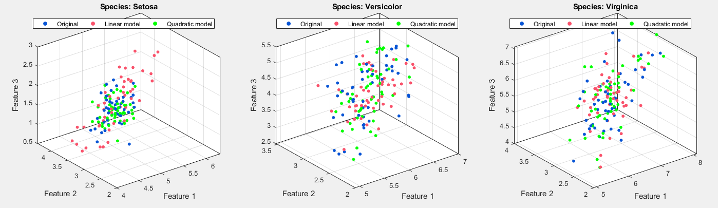
At last, we could graphically compare the generated samples, including generated by linear model and by quadratic model, and original ones:
1
2
3
4
5
6
7
8
9
10
11
12
13
14
15
16
17
18
19
20
21
22
23
24
25
26
27
28
29
30
31
32
33
34
35
36
37
38
39
40
41
42
43
44
45
46
47
48
49
50
51
52
53
54
55
56
57
58
59
60
61
62
63
64
65
66
67
68
69
70
71
72
clc,clear,close all

load fisheriris
meas = meas(:,1:3);

mdl_linear = fitcdiscr(meas,species); % DiscrimType: linear
mus_linear = mdl_linear.Mu;
Sigmas_linear = mdl_linear.Sigma;

mdl_quadratic = fitcdiscr(meas,species,"DiscrimType","quadratic"); % DiscrimType: quadratic
mus_quadratic = mdl_quadratic.Mu;
Sigmas_quadratic = mdl_quadratic.Sigma;

numNew = 50;

newSetosa_linear = mvnrnd(mus_linear(1,:),Sigmas_linear,numNew);
newSetosa_quadratic = mvnrnd(mus_quadratic(1,:),Sigmas_quadratic(:,:,1),numNew);

newVersicolor_linear = mvnrnd(mus_linear(2,:),Sigmas_linear,numNew);
newVersicolor_quadratic = mvnrnd(mus_quadratic(2,:),Sigmas_quadratic(:,:,2),numNew);

newVirginica_linear = mvnrnd(mus_linear(3,:),Sigmas_linear,numNew);
newVirginica_quadratic = mvnrnd(mus_quadratic(3,:),Sigmas_quadratic(:,:,3),numNew);

meas_setosa = meas(strcmp(species,"setosa"),:);
meas_versicolor = meas(strcmp(species,"versicolor"),:);
meas_virginica = meas(strcmp(species,"virginica"),:);

figure("Units","pixels","Position",[390.3333333333333,465,1550,420])
tiledlayout(1,3)
markerSize = 20;
nexttile
hold(gca,"on"),box(gca,"on"),grid(gca,"on"),view(3)
scatter3(meas_setosa(:,1),meas_setosa(:,2),meas_setosa(:,3), ...
    markerSize,"filled","DisplayName","Original","MarkerFaceColor",[7,84,213]/255)
scatter3(newSetosa_linear(:,1),newSetosa_linear(:,2),newSetosa_linear(:,3), ...
    markerSize,"filled","DisplayName","Linear model","MarkerFaceColor",[249,82,107]/255)
scatter3(newSetosa_quadratic(:,1),newSetosa_quadratic(:,2),newSetosa_quadratic(:,3), ...
    markerSize,"filled","DisplayName","Quadratic model","MarkerFaceColor","g")
legend("Location","northeast","Orientation","horizontal");
title("Species: Setosa")
xlabel("Feature 1")
ylabel("Feature 2")
zlabel("Feature 3")

nexttile
hold(gca,"on"),box(gca,"on"),grid(gca,"on"),view(3)
scatter3(meas_versicolor(:,1),meas_versicolor(:,2),meas_versicolor(:,3), ...
    markerSize,"filled","DisplayName","Original","MarkerFaceColor",[7,84,213]/255)
scatter3(newVersicolor_linear(:,1),newVersicolor_linear(:,2),newVersicolor_linear(:,3), ...
    markerSize,"filled","DisplayName","Linear model","MarkerFaceColor",[249,82,107]/255)
scatter3(newVersicolor_quadratic(:,1),newVersicolor_quadratic(:,2),newVersicolor_quadratic(:,3), ...
    markerSize,"filled","DisplayName","Quadratic model","MarkerFaceColor","g")
legend("Location","north","Orientation","horizontal");
title("Species: Versicolor")
xlabel("Feature 1")
ylabel("Feature 2")
zlabel("Feature 3")

nexttile
hold(gca,"on"),box(gca,"on"),grid(gca,"on"),view(3)
scatter3(meas_virginica(:,1),meas_virginica(:,2),meas_virginica(:,3), ...
    markerSize,"filled","DisplayName","Original","MarkerFaceColor",[7,84,213]/255)
scatter3(newVirginica_linear(:,1),newVirginica_linear(:,2),newVirginica_linear(:,3), ...
    markerSize,"filled","DisplayName","Linear model","MarkerFaceColor",[249,82,107]/255)
scatter3(newVirginica_quadratic(:,1),newVirginica_quadratic(:,2),newVirginica_quadratic(:,3), ...
    markerSize,"filled","DisplayName","Quadratic model","MarkerFaceColor","g")
legend("Location","northeast","Orientation","horizontal");
title("Species: Virginica")
xlabel("Feature 1")
ylabel("Feature 2")
zlabel("Feature 3")
We could simply test the similarity of generated samples and original ones by Mahalanobis Distance (could see blog [3]) for both models:
1
2
3
4
5
6
7
8
9
10
11
12
13
14
15
fprintf("Linear model, Avarage Mahalanobis distance: \n" + ...
    "(setosa): %.4f\n" + ...
    "(versicolor): %.4f\n" + ...
    "(Virginica): %.4f\n", ...
    mean((sqrt(mahal(newSetosa_linear,meas_setosa)))), ...
    mean((sqrt(mahal(newVersicolor_linear,meas_versicolor)))), ...
    mean((sqrt(mahal(newVirginica_linear,meas_virginica)))));
disp(newline)
fprintf("Quadratic model, Avarage Mahalanobis distance: \n" + ...
    "(setosa): %.4f\n" + ...
    "(versicolor): %.4f\n" + ...
    "(Virginica): %.4f\n", ...
    mean((sqrt(mahal(newSetosa_quadratic,meas_setosa)))), ...
    mean((sqrt(mahal(newVersicolor_quadratic,meas_versicolor)))), ...
    mean((sqrt(mahal(newVirginica_quadratic,meas_virginica)))));
1
2
3
4
5
6
7
8
9
Linear model, Avarage Mahalanobis distance:
(setosa): 2.8597
(versicolor): 1.6980
(Virginica): 1.4635

Quadratic model, Avarage Mahalanobis distance:
(setosa): 1.5988
(versicolor): 1.6957
(Virginica): 1.5438
In a word, for class setosa, quadratic model is better than linear model, while for other two classes, the performance of both model is similar.
Hyperparameter Optimizsation Options and Discussions
Actually, if see official documentation in detail [1], we could find that the fitcdiscr function actually support using cross validation to automatically optimise hyperparameters of the model. Some concerned arguments of fitcdiscr function are about this setting, and I think this is more complicated part of this function.
Most important, from the running results at this case, I speculate that the way of verification described above, that is moment estimation [4], is not appropriate. The fitcdiscr function more likely to solve a maximum likelihood estimation with regularisation.
And the similarity of mean vector and covariance matrix of the model and sample mean vector and sample covariance matrix is just a coincidence, which could refer to [4,5]. Another official documentation [6] gives more information about Discriminant Analysis Models, but I don’t plan to get into it at present since my original motivation of recording this function is that I found it unfamiliar in another official example [7]. Although the analysis content may be wrong (and with a high probability), I have known something about it. So, I decide to learn it more deeply if needed in the future.
References
[2] Gaussian Mixture Model(GMM) - What a starry night~.
[3] Multivariate Normal Distribution and Mahalanobis Distance - What a starry night~.
[4] Point Estimation - What a starry night~.
[5] Maximum Likelihood Estimation for Multivariate Normal Distribution - What a starry night~.
[6] Prediction Using Discriminant Analysis Models - MathWorks.