Physical System Modeling using LSTM Network in MATLAB Simulink
Introduction
MATLAB官方提供了一个使用LSTM神经网络实现物理仿真模型降阶的示例1:

This example shows how to create a reduced order model (ROM) to replace a Simscape component in a Simulink® model by training a long short-term memory (LSTM) neural network.
A ROM is a surrogate for a physical model that allows you to reduce the computation required without compromising the accuracy of the original physical model. For workflows that require heavy computations, such as design exploration, you can use the ROM in place of the original physical system. While there is a variety of techniques for building a ROM, this example builds an LSTM-ROM (a type of ROM that leverages an LSTM network) and uses it in a Simulink model as part of a Deep Learning Stateful Predict block.
To train the LSTM network, the example uses the original model to generate the training data. The trained LSTM in the ROM takes the B and F signals of the load shaft and the control pressure as input and predicts the next value of the B and F signals of the load shaft. After the model is trained, the example creates an LSTM-ROM component and replaces the physical component in the Simulink model with it.
Workflow
Generate training and test Data
训练集数据来自仿真文件ex_sdl_flexible_shaft.slx:

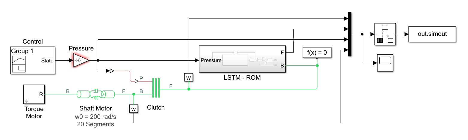
该Simulink文件仿真了一个flexible shaft(柔性轴)。它有两个柔性铝轴,分别是motor shaft和load shaft,使用集总参数方法(lumped parameter approach)建模。两个轴都包含inertias,damping和stiff torsional springs(刚性扭转弹簧)。
-
仿真开始时,clutch解锁,driven shaft(从动轴)自由;
-
motor shaft的初速度为200 rad/s,系统以稳定状态启动;
-
整个模型使用“施加在clutch上的pressure”作为control parameter决定模型的动态特性。
-
Simulink的模型有四个输出信号:
- load shaft的Base (B) signal(基本信号)
- load shaft的Follower (F) signal(跟随信号)
- Control pressure
- motor shaft的F signal
前三个信号用于训练LSTM-ROM,第四个信号用于评价训练整个模型的准确度。
我们通过下面的脚本文件控制Control pressure并进行仿真,获得数据集:
1
2
3
4
5
6
7
8
9
10
11
12
13
14
15
16
17
18
clc, clear, close all

stopTime = 0.2;  % stop time
timeInterval = 5e-5; % time interval

% The Pressure block of the model depends on the workspace variable maxPressure, which defines the value of the maximum pressure applied on the clutch.
% Run the model for 20 different equally spaced values of maxPressure between 10e5 and 10e6.
% Collect the output data in the cell array data, where each element corresponds to a time series observation computed with the specified pressure profile.
numObservations = 20;
maxPressures = linspace(1e5,1e6,numObservations);

data = cell(numObservations,1);

for i = 1:numObservations
    maxPressure = maxPressures(i);
    simout = sim("ex_sdl_flexible_shaft");
    data{i} = simout.simout.Data';
end
此时,变量data中就包含了20次仿真的输出信号:
1
2
3
4
5
6
7
8
9
10
11
12
13
14
15
16
17
18
19
20
21
22
23
>> data
data =
  20×1 cell array
    {4×4001 double}
    {4×4001 double}
    {4×4001 double}
    {4×4001 double}
    {4×4001 double}
    {4×4001 double}
    {4×4001 double}
    {4×4001 double}
    {4×4001 double}
    {4×4001 double}
    {4×4001 double}
    {4×4001 double}
    {4×4001 double}
    {4×4001 double}
    {4×4001 double}
    {4×4001 double}
    {4×4001 double}
    {4×4001 double}
    {4×4001 double}
    {4×4001 double}
之后,可以看一下输出的信号波形:
1
2
3
4
5
6
7
8
9
10
11
12
13
14
15
16
17
18
19
20
21
22
23
24
25
26
27
28
29
30
31
32
% Extract the time steps of the simulations
times = simout.simout.Time;
numTimeSteps = length(times);

figure("Units", "pixels", "Position", [244,262,1006,363])
tiledlayout(1,2)

% Plot the control pressures of the first five simulations.
nexttile
hold(gca, "on")
box(gca, "on")
for i = 1:5
    pressure = data{i}(3,:);
    plot(times, pressure, LineWidth=1.5);
end
title("Input Pressure")
legend("Observation " + (1:5))
xlabel("Time")
ylabel("Pressure (Pa)")


% Plot the B and F signals of the load shaft and the F signal of the motor shaft of one of the simulations.
nexttile
idx = 4;
BLoadShaft = data{idx}(1,:);
FLoadShaft = data{idx}(2,:);
FMotorShaft = data{idx}(4,:);
plot(times,BLoadShaft, ...
    times,FLoadShaft, ...
    times,FMotorShaft)
% legend("B - Load Shaft", "F - Load Shaft", "F - Motor Shaft")
title("Model Dynamics (Maximum Pressure =  " + maxPressures(idx) + " Pa)")

为了看得清楚一点,我们将三个信号分别画出来:
1
2
3
4
5
6
7
8
9
10
11
12
13
14
15
16
17
18
19
figure("Units", "pixels", "Position", [353,408,1145,268])
tiledlayout(1,3)
yLimits = [0, 250];

nexttile
plot(times, BLoadShaft, LineWidth=1.5)
ylim(yLimits)
legend("B - Load Shaft")

nexttile
plot(times, FLoadShaft, LineWidth=1.5)
ylim(yLimits)
legend("F - Load Shaft")

nexttile
plot(times, FMotorShaft, LineWidth=1.5)
ylim(yLimits)
legend("F - Motor Shaft")
exportgraphics(gcf, "fig-2.jpg", Resolution=600)

之后,我们将变量data保存,以供后续使用:
1
2
% Save output signals
save("data.mat", "data")
Prepare data for training (downsample signals)
如果使用非常长的数据序列训练LSTM,每一个时间步长所计算的梯度的累积可能会导致梯度消失,使得训练过程收敛到次优的(suboptimal)结果。为了避免梯度消失,我们对训练数据进行下采样(downsample),在不损失太多信息的情况下压缩序列的长度。
1
2
3
4
5
6
7
8
9
10
11
12
13
14
15
clc, clear, close all

load data.mat

timeInterval = 5e-5;
numObservations = 20;
numTimeSteps = length(times);

% Prepare data for training
sampleTime = 1e-3;
intervalDownsampled = sampleTime / timeInterval;
timeStepsDownsampled = 1:intervalDownsampled:numTimeSteps;
for i = 1:numObservations
    dataDownsampled{i} = data{i}(:,timeStepsDownsampled);
end
此时,原本4001个采样点的信号被下采样至201个采样点:
1
2
3
>> size(dataDownsampled{1})
ans =
     4   201
Partition dataset
之后,使用该示例自带的函数文件trainingPartitions.m划分数据集为训练集和测试集:
1
2
3
4
5
6
7
8
9
10
11
12
13
14
15
16
17
18
19
20
21
22
23
24
25
26
27
28
29
30
31
32
33
34
35
36
37
38
39
40
41
42
43
44
45
46
47
function varargout = trainingPartitions(numObservations,splits)
%TRAININGPARTITONS Random indices for splitting training data
%   [idx1,...,idxN] = trainingPartitions(numObservations,splits) returns
%   random vectors of indices to help split a data set with the specified
%   number of observations, where SPLITS is a vector of length N of
%   partition sizes that sum to one.
%
%   Example: Get indices for 50%-50% training-test split of 500
%   observations.
%   [idxTrain,idxTest] = trainingPartitions(500,[0.5 0.5])
%
%   Example: Get indices for 80%-10%-10% training, validation, test split
%   of 500 observations.
%   [idxTrain,idxValidation,idxTest] = trainingPartitions(500,[0.8 0.1 0.1])

arguments
    numObservations (1,1) {mustBePositive}
    splits {mustBeVector,mustBeInRange(splits,0,1,"exclusive"),mustSumToOne}
end

numPartitions = numel(splits);
varargout = cell(1,numPartitions);

idx = randperm(numObservations);

idxEnd = 0;

for i = 1:numPartitions-1
    idxStart = idxEnd + 1;
    idxEnd = idxStart + floor(splits(i)*numObservations) - 1;

    varargout{i} = idx(idxStart:idxEnd);
end

% Last partition.
varargout{end} = idx(idxEnd+1:end);

end

function mustSumToOne(v)
% Validate that value sums to one.

if sum(v,"all") ~= 1
    error("Value must sum to one.")
end

end
划分数据集代码:
1
2
3
4
5
6
7
% Partition the training data evenly into training and test partitions using the trainingPartitions function
[idxTrain, idxTest] = trainingPartitions(numObservations, [0.5 0.5]);

maxPressuresTrain = maxPressures(idxTrain);
maxPressuresTest = maxPressures(idxTest);
dataTrain = dataDownsampled(idxTrain);
dataTest = dataDownsampled(idxTest);
在这个示例中,训练集和测试集的各有10条。
Predictors and targets of LSTM
之后我们从training data中提取predictors和targets。其中,predictors由三部分组成:
- load shaft的B signals
- load shaft的F signals
- control pressure
这三个predictors对应变量dataTrain的前三个通道。targets对应dataTrain每一个cell的前两个通道偏移1个时间步长的值:
1
2
3
4
5
6
7
8
inputStatesTrain  = [1 2 3];
outputStatesTrain = [1 2];

numObservationsTrain = numel(dataTrain);
for i = 1:numObservationsTrain
    XTrain{i} = dataTrain{i}(inputStatesTrain,1:end-1);
    TTrain{i} = dataTrain{i}(outputStatesTrain,2:end);
end
Define network architecture
这部分定义LSTM的结构:
Define the following LSTM network, which predicts the next B and F signal values.
- For sequence input, specify a sequence input layer with an input size matching the number of inputs. Normalize the inputs by rescaling them to have values between zero and one.
- To learn interactions between the input features, include a fully connected layer with an output size of 200 followed by a ReLU layer.
- To learn long-term dependencies in the sequence data, include two LSTM layers with 200 hidden units followed by a ReLU layer.
- To output predictions of the correct size, include a fully connected layer with a size matching the number of responses.
- To train the network for regression, include a regression layer.
1
2
3
4
5
6
7
8
9
10
11
12
13
14
15
16
17
18
tnumHiddenUnits = 200;

numFeatures = numel(inputStatesTrain);
numResponses = numel(outputStatesTrain);

layers = [
    sequenceInputLayer(numFeatures,Normalization="rescale-zero-one")

    fullyConnectedLayer(numHiddenUnits)
    reluLayer

    lstmLayer(numHiddenUnits)
    lstmLayer(numHiddenUnits)
    reluLayer

    fullyConnectedLayer(numResponses)

    regressionLayer];
需要注意的一点是,我们这里训练的是一个回归模型。
Specify training options and train LSTM Network
1
2
3
4
5
6
7
8
9
10
11
12
13
options = trainingOptions("adam", ...
    MaxEpochs=3e4, ...
    GradientThreshold=1, ...
    InitialLearnRate=5e-3, ...
    LearnRateSchedule="piecewise", ...
    LearnRateDropPeriod=1e4, ...
    LearnRateDropFactor=0.6, ...
    Verbose=0, ...
    Plots="training-progress");
net = trainNetwork(XTrain, TTrain, layers, options);

filename = "flexibleShaftLoadNet.mat";
save(filename,"net")
最后,保存一下测试集的信息,以供后续测试模型时使用:
1
save("test.mat", "dataTest", "maxPressuresTest")
LSTM-ROM in Simulink model
该实例提供了使用上述LSTM神经网络的Simulink模型:ex_sdl_flexible_shaft_lstm.slx。
该模型中的子部件LSTM-ROM:

该子部件:
- outputs the predicted B and F signals of the load shaft using a trained LSTM network.
- The block uses the predictions for the next time step through a feedback loop.
并在子模块中设置trained network的位置和sample time。

这个子模块Stateful Predict2 是MATLAB Simulink提供的模块,来自Deep Learning Toolbox / Deep Neural Networks库。这个库中还具有以下几类模块:

Test model
最后,我们使用held-out test data测试模型。需要注意的是,我们在这里测试的是full model,而非just the LSTM network,而用于测试对比的信号是motor shaft的F signals。
首先,我们从test data中提取targets。
The test targets are simulated F signals of the motor shaft using the original model, shifted by one time step.
1
2
3
4
5
6
7
numObservationsTest = numel(dataTest);

outputStatesTest = 4;

for i = 1:numObservationsTest
    TTest{i} = dataTest{i}(outputStatesTest,2:end);
end
对于每一个test dataset中的数据所对应的maximum pressure value,都运行一次仿真模型(具有LSTM-ROM模型),并且保存motor shaft的F signals。
1
2
3
4
5
6
7
errs = [];
for i = 1:numObservationsTest
    maxPressure = maxPressuresTest(i);
    simout = sim("ex_sdl_flexible_shaft_lstm");

    YTest{i} = simout.simout.Data(1:end-1,4)';
end
注:运行包含LSTM的Simulink模型遇到了各种各样的讲稿和错误,调试的具体过程放在文末的Appendix中。
另外需要注意的是,为了学习方便,我将整个示例的代码分割成三部分,因此在测试模型之前需要再加载一下前面的数据和参数。比如前面保存的测试集数据:
1
load test.mat
和Simulink模型运行所需的参数:
1
2
stopTime = 0.2;
sampleTime = 1e-3;
以及物理仿真模型ex_sdl_flexible_shaft.slx中预加载的模型参数:
1
2
3
4
5
6
7
8
9
10
11
12
13
14
% Shaft properties
fShaft.Material = 'Aluminum Alloy';
fShaft.ShearModulus = 26E9;
fShaft.Diameter = 0.025;
fShaft.Length = 5;
fShaft.Density = 2.7E3;
fShaft.DampingCoeff = 0.02;

% Derived properties
fShaft.Stiffness = pi/32 * (fShaft.Diameter)^4 ...
    * fShaft.ShearModulus / fShaft.Length;

fShaft.Inertia = pi/32 * (fShaft.Diameter)^4 ...
    * fShaft.Density * fShaft.Length ;
最终,可视化:
- 真实信号与预测信号之间的差异(测试对比信号:motor shaft的F signals);
- step predictions in scatter plot;
- prediction errors in histogram;
1
2
3
4
5
6
7
8
9
10
11
12
13
14
15
16
17
18
19
20
21
22
23
24
25
26
27
28
29
Real = [TTest{:}];
Pred = [YTest{:}];

figure("Units", "pixels", "Position", [248,294,1289,339])
tiledlayout(1,3)
nexttile
hold(gca, "on")
box(gca, "on")
plot(1:numel(Real), Real, DisplayName="Real signals")
plot(1:numel(Pred), Pred, DisplayName="Predicted signals")
legend
xlabel("Sample points")

nexttile
hold(gca, "on")
box(gca, "on")
scatter(Real, Pred)
m = min([Real, Pred]);
M = max([Real, Pred]);
plot([m M],[m M],"r--")
xlabel("Target")
ylabel("Prediction")
xlim([m M])
ylim([m M])

nexttile
histogram(Real-Pred)
xlabel("Error")
ylabel("Frequency")

Conclusion
最后,我们总结上述过程。首先,我们将不同的Maximum pressure传入到纯物理Simulink模型中,得到四个信号输出:

我们将得到的数据集切分为训练集和测试集(注意:此时的训练集和测试集都包含Maximum pressure和四个信号),按照下面的示意图所示提取出训练集的predictors XTrain和targets TTrain以训练LSTM。之后在Simulink中将LSTM与物理模型融合,得到具有LSTM-ROM的物理模型。然后,我们将测试集中的Maximum pressure输入到新的模型中,得到测试集标签YTest,将YTest与相同Maximum pressure对应的TTest信号做对比,以验证具有深度神经网络模型的物理模型的性能:

在整个过程中我们可以看到,用于测试模型性能所采用的信号(信号4)与训练LSTM所采用的信号(信号1~3)是不一致的,我个人认为这一点是可以理解的,因为文档原文中有提到:
To test the accuracy of the full model, not just the LSTM network, compare the outputs with the simulated F signals of the motor shaft generated by the original Simulink model.
也就是说,我们在这里并不是主要关心LSTM模型的性能是怎样的(是否过拟合等等),而是关注整个模型的性能。我们当然也可以考察一下LSTM模型信号1~2的输出,但是信号4可能是这个模型最为关心的输出信号。
另外,我们还可以看到我们用于对比的真实信号TTest和模型输出的信号YTest差了一个步长,这一点也是代码编写人员有意而为之的:
Extract the targets from the test data. The test targets are simulated F signals of the motor shaft using the original model, shifted by one time step.
因为新的Simulink使用了LSTM-ROM模块:

文档中提到说,该模块:
The block uses the predictions for the next time step through a feedback loop.
对于仿真中步长级别的差异我不是很清楚,我感觉可能是因为这个原因。
我也尝试了不考虑这一个步长的shift,让两个信号完全对齐来测试,发现两种测试方法得到的结果之间的差异微乎其微微乎其微。因此在实践中,这一个步长的差别可以忽略不计。
Appendix
在测试含有ROM-LSTM的Simulink模型时,即运行代码片段:
1
2
3
4
5
6
for i = 1:numObservationsTest
    maxPressure = maxPressuresTest(i);
    simout = sim("ex_sdl_flexible_shaft_lstm");

    YTest{i} = simout.simout.Data(1:end-1,4)';
end
出现了一系列不同的报错,总体上可以概括为:
- MEX complier不正确
- Explicit solver输入参数不足
- 缺乏GPU Coder Interface for Deep Learning Libraries
- GPU驱动版本
第一次运行程序,出现了下面的报错:
1
2
3
4
> In script3_test_model (line 34)
Error using script3_test_model
Selected MEX compiler 'mingw64-g++' is not supported for GPU code generation. Refer to the GPU Coder documentation for a list of supported GPU MEX
compilers.
报错的原因是电脑所使用的编译器不在supported GPU MEX的名单中。MATLAB Answers中一则Q&A提到了类似的问题3,Roberson的建议是需要将Visual Sutio作为GPU coder的编译器。于是我就下载了2022版本的Microsoft Visual Studio。再次运行时,则出现了另一个报错:
1
2
3
4
5
6
Error using script3_test_model
Unable to create mex function 'ex_sdl_flexible_shaft_lstm_sfun.mexw64' required for simulation.

C:\Program Files\MATLAB\R2022a\sys\cuda\win64\cuda\include\crt/host_config.h(160): fatal error C1189: #error:  -- unsupported Microsoft Visual Studio version! Only the versions between 2017 and 2019 (inclusive) are supported! The nvcc flag '-allow-unsupported-compiler' can be used to override this version check; however, using an unsupported host compiler may cause compilation failure or incorrect run time execution. Use at your own risk.
nvcc warning : The 'compute_35', 'compute_37', 'compute_50', 'sm_35', 'sm_37' and 'sm_50' architectures are deprecated, and may be removed in a future release (Use -Wno-deprecated-gpu-targets to suppress warning).
ex_sdl_flexible_shaft_lstm_sfun.cu
错误的原因是:Microsoft Visual Studio 2022并不是所支持的版本,需要使用2017至2019年之间的版本。于是,我就删除了2022的版本,又下载了2019版。再次运行后,又出现了新的报错:
1
2
3
4
5
6
7
8
9
10
11
12
13
14
15
16
17
18
19
20
21
22
23
24
25
26
27
28
29
30
31
32
33
34
35
Warning: The file containing block diagram 'ex_sdl_flexible_shaft_lstm' is shadowed by a file of the same name higher on the MATLAB
path. This can cause unexpected behavior. For more information see "Avoiding Problems with Shadowed Files" in the Simulink
documentation.

The file containing the block diagram is:
C:\Users\Tsing\Desktop\QinghuaMa.github.io\_drafts\2022.12.29\ex_sdl_flexible_shaft_lstm.slx.
The file higher on the MATLAB path is: C:\Users\Tsing\Desktop\test\ex_sdl_flexible_shaft_lstm.slx
Warning: This Simscape(TM) model contains both dynamic and algebraic equations even after model simplification. To improve
performance and robustness for this class of model an implicit solver is recommended.
Suggested Actions:
    • Choose an implicit solver. - Fix
    • To disable this diagnostic, set the  Explicit solver used in model containing Physical Networks blocks diagnostic to 'none'. -
    Apply

Error due to multiple causes.
Caused by:
    ['ex_sdl_flexible_shaft_lstm']: Not enough input derivatives were provided for one or more Simulink-PS Converter blocks for the
    solver chosen. Implicit solvers (ode23t, ode15s, and ode14x) typically require fewer input derivatives than explicit solvers, and
    local solvers never require any.

    The following Simulink-PS Converter blocks have piecewise constant inputs. To provide the derivatives required, you can either turn
    input filtering on, provide the input derivatives explicitly, or set them to zero by selecting the corresponding options on the
    Input Handling tab:

    ...'ex_sdl_flexible_shaft_lstm/LSTM - ROM/Simulink-PS
    Converter4' (2 required, 1 provided)

    The following Simulink-PS Converter blocks have continuous inputs. To provide the derivatives required, you can either turn input
    filtering on or provide the input derivatives explicitly by selecting the corresponding options on the Input Handling tab:

    ...'ex_sdl_flexible_shaft_lstm/Simulink-PS
    Converter' (1 required, 0 provided)
    Error generated while running CUDA-enabled program: [3,cudaErrorInitializationError] initialization error. To generate additional
    debugging information, enable the 'SimGPUErrorChecks' GPU code generation option.
    	Error in 'ex_sdl_flexible_shaft_lstm/LSTM - ROM/LSTM Network - Stateful Predict/MLFB'.
这次报错是求解器的报错,大致的意思是目前所采用的explicit求解器时输入数量不足,可能需要采用implicit。于是,我就进入到模型ex_sdl_flexible_shaft_lstm.slx的设置中,将求解器改为了auto:

再次运行后,软件又报了另外一个错误:

1
2
3
4
5
6
7
Error due to multiple causes.
Caused by:
    There is a problem with the graphics driver or with this GPU device. For more information on GPU support, see GPU Support by
    Release.
    Error generated while running CUDA-enabled program: [3,cudaErrorInitializationError] initialization error. To generate additional
    debugging information, enable the 'SimGPUErrorChecks' GPU code generation option.
    	Error in 'ex_sdl_flexible_shaft_lstm/LSTM - ROM/LSTM Network - Stateful Predict/MLFB'.
意思是MATLAB软件缺乏GPU Coder Interface for Deep Learning Libraries,需要到Add-On Explorer中进行下载:

但是也可以看到,再次运行后也仅仅是解决了上述的warning,相同的error仍然存在:

点开上图中GPU Support by Release的链接,可以看到,出现这个错误可能是因为电脑的GPU能用于MATLAB计算。
因为学校放假,我现在只能使用笔记本来运行这些代码。我手上这台笔记本有一块集成显卡(Inter(R) HD Graphics 630):

一块独立显卡(NVIDIA Geforce GTX 1050):

之前我一直以为集显肯定是不支持MATLAB计算的,但实际上这两块GPU都是无法用于MATLAB计算:
1
2
3
4
>> tf = canUseGPU()
tf =
  logical
   0
进一步地,如果尝试使用gpuDevice调用GPU,则会出现下面的报错:
1
2
3
4
5
>> gpuDevice
Error using gpuDevice
Graphics driver version 9.2 is not supported. Update graphics
driver to version 11.2 or greater. For more information on GPU
support, see GPU Support by Release.
所以,升级驱动可能会解决这一问题4。
在桌面右键点击NVIDIA 控制面板,再点击软件左下角的系统信息,可以看到GPU的详细信息:

可以看到GPU型号是GeForce GTX 1050,此时的驱动程序版本是:398.36。
我们到NVIDIA官网5,选择合适的驱动程序并下载:


此时,电脑重启后打开NVIDIA控制面板,可以看到驱动已经升级成功:

此时,再打开MATLAB查看一下GPU是否可以使用:
1
2
3
4
>> canUseGPU
ans =
  logical
   1
1
2
3
4
5
6
7
8
9
10
11
12
13
14
15
16
17
18
19
20
21
22
23
24
25
26
>> gpuDevice
ans =
  CUDADevice with properties:

                      Name: 'NVIDIA GeForce GTX 1050'
                     Index: 1
         ComputeCapability: '6.1'
            SupportsDouble: 1
             DriverVersion: 12
            ToolkitVersion: 11.2000
        MaxThreadsPerBlock: 1024
          MaxShmemPerBlock: 49152
        MaxThreadBlockSize: [1024 1024 64]
               MaxGridSize: [2.1475e+09 65535 65535]
                 SIMDWidth: 32
               TotalMemory: 4.2948e+09
           AvailableMemory: 3.4265e+09
       MultiprocessorCount: 5
              ClockRateKHz: 1493000
               ComputeMode: 'Default'
      GPUOverlapsTransfers: 1
    KernelExecutionTimeout: 1
          CanMapHostMemory: 1
           DeviceSupported: 1
           DeviceAvailable: 1
            DeviceSelected: 1
bingo~ 之后就可以运行啦~~
Reference