Dykstra’s Projection Algorithm
Introduction
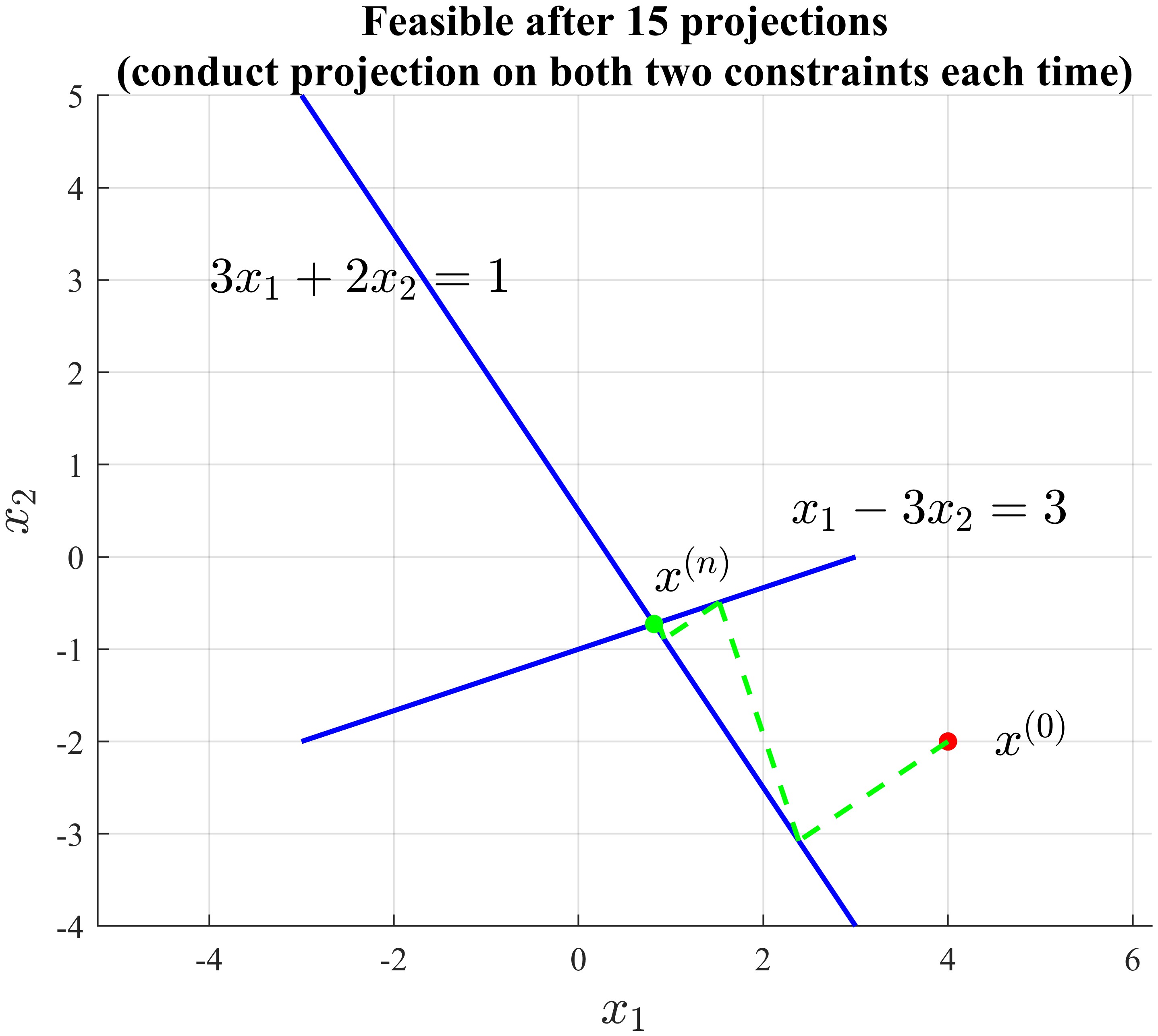
One of my previous blog1 ever discussed a problem of projecting $\boldsymbol{x}_0$ on such a halfspace:
\[\begin{split} \min_\boldsymbol{x}\,&\frac12||\boldsymbol{x}-\boldsymbol{x}_0||^2_{_2}\\ \text{s.t.} \,&\begin{bmatrix} 3 & 2 \\ 1 & -3\\ \end{bmatrix} \begin{bmatrix} x_1 \\ x_2 \end{bmatrix} \preceq \begin{bmatrix} 1 \\ 3 \end{bmatrix} \end{split}\label{eq2}\]and the POCS algorithm1 solves it well:
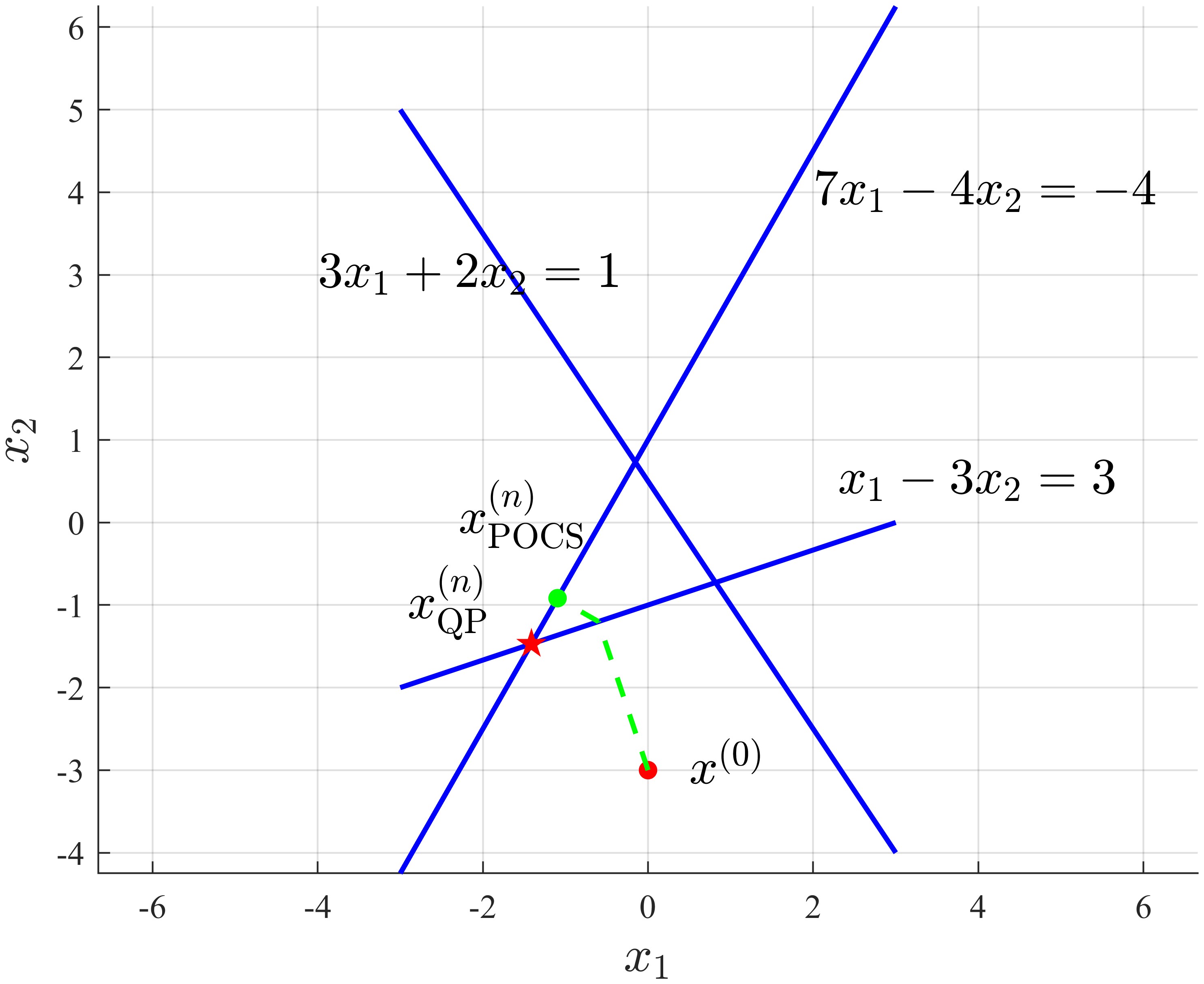
If we add another hyperplane to form a new polyhedron, i.e.,
\[\begin{split} \min_\boldsymbol{x}\,&\frac12||\boldsymbol{x}-\boldsymbol{x}_0||^2_{_2}\\ \text{s.t.} \,&\begin{bmatrix} 3 & 2 \\ 1 & -3\\ 7 & -4 \end{bmatrix} \begin{bmatrix} x_1 \\ x_2 \end{bmatrix} \preceq \begin{bmatrix} 1 \\ 3 \\ -4 \end{bmatrix} \end{split}\label{eq3}\]At this time, if we still use POCS, and compare with directly solving $\eqref{eq3}$ by MATLAB quadprog function (initial point $\boldsymbol{x}^{(0)}=[0,-3]^T$):
1
2
3
4
5
6
7
8
9
10
11
12
13
14
15
16
17
18
19
20
21
22
23
24
25
26
27
28
29
30
31
32
33
34
35
36
37
38
39
40
41
42
43
44
45
46
47
48
49
50
51
52
53
54
55
56
57
58
59
60
61
62
63
64
65
66
67
68
69
70
71
72
73
74
75
76
77
78
79
clc, clear, close all

x1 = linspace(-3, 3, 200);
a = [3, 1, 7;
    2, -3, -4];
b = [1; 3; -4];

figure('Color', 'w')
hold(gca, 'on')
grid(gca, 'on')
plot(x1, (1-3*x1)/2, 'LineWidth', 1.5, 'Color', 'b', 'HandleVisibility', 'off')
text(-4, 3, '$3x_1+2x_2=1$', 'Interpreter', 'latex', 'FontSize', 15)
plot(x1, (1/3)*x1-1, 'LineWidth', 1.5, 'Color', 'b', 'HandleVisibility', 'off')
text(2.3, 0.5, '$x_1-3x_2=3$', 'Interpreter', 'latex', 'FontSize', 15)
plot(x1, x1/(4/7)+1, 'LineWidth', 1.5, 'Color', 'b', 'HandleVisibility', 'off')
text(2, 4, '$7x_1-4x_2=-4$', 'Interpreter', 'latex', 'FontSize', 15)
axis('equal')

x0 = [0; -3];
scatter(x0(1), x0(2), 30, 'filled', 'MarkerFaceColor', 'r', 'HandleVisibility', 'off')
text(x0(1)+0.5, x0(2), '$x^{(0)}$', 'Interpreter', 'latex', 'FontSize', 15)

ntimes = 0;
while ~all(a'*x0 <= b)
    x_Pc1 = helperProjec(a(:,1), b(1), x0);
    plot([x0(1), x_Pc1(1)], [x0(2), x_Pc1(2)], 'LineWidth', 1.5, 'Color', 'g', 'LineStyle', '--', 'HandleVisibility', 'off')

    if all(a'*x_Pc1 <= b)
        x_projection = x_Pc1;
        ntimes = ntimes+1;
        break
    end

    x_Pc2 = helperProjec(a(:,2), b(2), x_Pc1);
    plot([x_Pc1(1), x_Pc2(1)], [x_Pc1(2), x_Pc2(2)], 'LineWidth', 1.5, 'Color', 'g', 'LineStyle', '--', 'HandleVisibility', 'off')

    if all(a'*x_Pc2 <= b)
        x_projection = x_Pc2;
        ntimes = ntimes+1;
        break
    end

    x_Pc3 = helperProjec(a(:,3), b(3), x_Pc2);
    plot([x_Pc2(1), x_Pc3(1)], [x_Pc2(2), x_Pc3(2)], 'LineWidth', 1.5, 'Color', 'g', 'LineStyle', '--', 'HandleVisibility', 'off')

    if all(a'*x_Pc3 <= b)
        x_projection = x_Pc3;
        ntimes = ntimes+1;
        break
    end

    x0 = x_Pc3;
    ntimes = ntimes+1;
end

x_qp = quadprog(eye(2) , -x0, a', b);

scatter(x_projection(1), x_projection(2), 30, 'filled', 'MarkerFaceColor', 'g', 'HandleVisibility', 'off')
text(x_projection(1)-1.2, x_projection(2)+1, '$x^{(n)}_\mathrm{POCS}$', 'Interpreter', 'latex', 'FontSize', 15)
fprintf('Solution by POCS: (%.4f, %.4f)\n', x_projection(1), x_projection(2))

scatter(x_qp(1), x_qp(2), 90, 'filled', 'Marker', 'pentagram', 'MarkerFaceColor', 'r', 'HandleVisibility', 'off')
text(x_qp(1)-1.5, x_qp(2)+0.5, '$x^{(n)}_\mathrm{QP}$', 'Interpreter', 'latex', 'FontSize', 15)
fprintf('Solution by solving QP: (%.4f, %.4f)\n', x_qp(1), x_qp(2))

legend('Box', 'off', 'FontSize', 15)
xlabel('$x_1$', 'Interpreter', 'latex', 'FontSize', 15)
ylabel('$x_2$', 'Interpreter', 'latex', 'FontSize', 15)
set(gca, 'FontName', 'Times New Roman')

exportgraphics(gca, 'fig1.jpg', 'Resolution', 600)

function x_pc = helperProjec(a, b, x0)
if a'*x0<=b
    x_pc = x0;
else
    x_pc = x0+(b-a'*x0)*a/norm(a)^2;
end
end
1
2
Solution by POCS: (-1.0954, -0.9169)
Solution by solving QP: (-1.4118, -1.4706)
At this time, we can see the point that POCS found is not the QP’s solution, meaning that, even if POCS can find a point in the feasible domain, it can’t guarantee the point is the one whose distance from initial point $\boldsymbol{x}^{(0)}$ is the least, i.e., the point is not necessarily the solution of corresponding QP. So, we should turn to Dykstra’s projection algorithm.
Dykstra’s projection algorithm
Two-set case
The Dykstra’s projection algorithm is2:
Dykstra’s algorithm finds for each $\boldsymbol{r}$ the only $\bar{\boldsymbol{x}}\in C\cap D$ such that:
\[\vert\vert\bar{\boldsymbol{x}}-\boldsymbol{r}\vert\vert^2\le\vert\vert\boldsymbol{x}-\boldsymbol{r}\vert\vert^2,\,\text{for all }\boldsymbol{x}\in C\cap D\]where $C$, $D$ are convex sets. This problem is equivalent to finding the projection of $\boldsymbol{r}$ onto the set $C\cap D$ (btw, this is actually the meaning of original QP1), which we denote by $\mathcal{P}_{C\cap D}$.
To use Dykstra’s algorithm, one must know how to project onto the sets $C$ and $D$ separately.
First, consider the basic alternating projection (aka POCS) method (first studied, in the case when the sets $C$, $D$ were linear subspaces, by John von Neumann, which initializes $\boldsymbol{x}_0=\boldsymbol{r}$ and then generates the sequence:
\[\boldsymbol{x}_{k+1} = \mathcal{P}_C(\mathcal{P}_D(\boldsymbol{x}_k))\label{eq9}\]Dykstra’s algorithm is of a similar form, but uses additional auxiliary variables. Start with $\boldsymbol{x}_0 = \boldsymbol{r}$, $\boldsymbol{p}_0 = \boldsymbol{q}_0 = \boldsymbol{0}$ and update by:
\[\begin{split} &\boldsymbol{y}_k = \mathcal{P}_D(\boldsymbol{x}_k+\boldsymbol{p}_k)\\ &\boldsymbol{p}_{k+1} = \boldsymbol{x}_k+\boldsymbol{p}_k-\boldsymbol{y}_k\\ &\boldsymbol{x}_{k+1} = \mathcal{P}_C(\boldsymbol{y}_k+\boldsymbol{q}_k)\\ &\boldsymbol{q}_{k+1} = \boldsymbol{y}_k+\boldsymbol{q}_k-\boldsymbol{x}_{k+1}\\ \end{split}\label{eq1}\]Then the sequence ($\boldsymbol{x}_k$) converges to the solution of the original problem.

In the update formula $\eqref{eq1}$:
- $\boldsymbol{x}$ is the variable to be solved (here, in the $k$-th iteration, \(\boldsymbol{x}_k\) denotes the starting point before projection, and \(\boldsymbol{x}_{k+1}\) is the point we get after $k$-th iteration),
- $\boldsymbol{y}$ is an intermediate variable (representing the intermediate projection point),
- $\boldsymbol{p}$ and $\boldsymbol{q}$ are auxiliary variables.
If we first eliminate variable $\boldsymbol{y}_k$ in $\eqref{eq1}$:
\[\begin{split} &\boldsymbol{p}_{k+1} = \boldsymbol{x}_k+\boldsymbol{p}_k-\mathcal{P}_D(\boldsymbol{x}_k+\boldsymbol{p}_k)\\ &\boldsymbol{x}_{k+1} = \mathcal{P}_C(\mathcal{P}_D(\boldsymbol{x}_k+\boldsymbol{p}_k)+\boldsymbol{q}_k)\\ &\boldsymbol{q}_{k+1} = \mathcal{P}_D(\boldsymbol{x}_k+\boldsymbol{p}_k)+\boldsymbol{q}_k-\boldsymbol{x}_{k+1}\\ \end{split}\label{eq8}\]and then bring the second equation in $\eqref{eq8}$ into third equation:
\[\begin{split} &\boldsymbol{p}_{k+1} = \boldsymbol{x}_k+\boldsymbol{p}_k-\mathcal{P}_D(\boldsymbol{x}_k+\boldsymbol{p}_k)\\ &\boldsymbol{x}_{k+1} = \mathcal{P}_C(\mathcal{P}_D(\boldsymbol{x}_k+\boldsymbol{p}_k)+\boldsymbol{q}_k)\\ &\boldsymbol{q}_{k+1} = \mathcal{P}_D(\boldsymbol{x}_k+\boldsymbol{p}_k)+\boldsymbol{q}_k-\mathcal{P}_C(\mathcal{P}_D(\boldsymbol{x}_k+\boldsymbol{p}_k)+\boldsymbol{q}_k)\\ \end{split}\]we’ll see if auxiliar variables $\boldsymbol{p}$ and $\boldsymbol{q}$ are always zero vectors (and hence no need to update), this is actually original POCS $\eqref{eq9}$.
Multi-set case
Update formula $\eqref{eq1}$ shows the case of two sets $C$ and $D$. To step future, we can generalize it to multiple-set case.
First, in $\eqref{eq1}$, re-denote the sets $C$ and $D$ using a unified symbol $C_i$:
\[\begin{split} &\boldsymbol{y}_k = \mathcal{P}_{C_1}(\boldsymbol{x}_k+\boldsymbol{p}_k)\\ &\boldsymbol{p}_{k+1} = \boldsymbol{x}_k+\boldsymbol{p}_k-\boldsymbol{y}_k\\ &\boldsymbol{x}_{k+1} = \mathcal{P}_{C_2}(\boldsymbol{y}_k+\boldsymbol{q}_k)\\ &\boldsymbol{q}_{k+1} = \boldsymbol{y}_k+\boldsymbol{q}_k-\boldsymbol{x}_{k+1}\\ \end{split}\label{eq4}\]Next, let’s denote the first point (the starting point before projection) in the $k$-th iteration as $\boldsymbol{u}_0^{(k)}$ (note here we use superscript $(k)$ to represent the $k$-th iteration), the projection point on the first set $C_1$ as $\boldsymbol{u}_1^{(k)}$, the projection point on the second set $C_2$ as $\boldsymbol{u}_2^{(k)}$ , i.e., in the two-set case:
\[\boldsymbol{u}_0^{(k)}:=\boldsymbol{x}_{k},\, \boldsymbol{u}_1^{(k)}:=\boldsymbol{y}_{k},\, \boldsymbol{u}_2^{(k)}:=\boldsymbol{x}_{k+1}\]then Eq. $\eqref{eq4}$ can be re-written as:
\[\begin{split} &\boldsymbol{u}_1^{(k)} = \mathcal{P}_{C_1}(\boldsymbol{u}_0^{(k)}+\boldsymbol{p}_k)\\ &\boldsymbol{p}_{k+1} = \boldsymbol{u}_0^{(k)}+\boldsymbol{p}_k-\boldsymbol{u}_1^{(k)}\\ &\boldsymbol{u}_2^{(k)} = \mathcal{P}_{C_2}(\boldsymbol{u}_1^{(k)}+\boldsymbol{q}_k)\\ &\boldsymbol{q}_{k+1} = \boldsymbol{u}_1^{(k)}+\boldsymbol{q}_k-\boldsymbol{u}_2^{(k)}\\ \end{split}\label{eq5}\]Next, replace the symbol of auxiliar variables — let $\boldsymbol{z}_i^{(k)}$ denote the auxiliar variable of $i$-th set, which has been updated in the $k$-th iteration. So, we have:
\[\boldsymbol{z}_1^{(k)} := \boldsymbol{p}_{k+1},\, \boldsymbol{z}_2^{(k)} := \boldsymbol{q}_{k+1}\]and for results of previous iteration, we use superscript $(k-1)$ to distinguish:
\[\boldsymbol{z}_1^{(k-1)} := \boldsymbol{p}_k,\, \boldsymbol{z}_2^{(k-1)} := \boldsymbol{q}_{k}\]So, $\eqref{eq5}$ will become:
\[\begin{split} &\boldsymbol{u}_1^{(k)} = \mathcal{P}_{C_1}(\boldsymbol{u}_0^{(k)}+\boldsymbol{z}_1^{(k-1)})\\ &\boldsymbol{z}_1^{(k)} = \boldsymbol{u}_0^{(k)}+\boldsymbol{z}_1^{(k-1)}-\boldsymbol{u}_1^{(k)}\\ &\boldsymbol{u}_2^{(k)} = \mathcal{P}_{C_2}(\boldsymbol{u}_1^{(k)}+\boldsymbol{z}_2^{(k-1)})\\ &\boldsymbol{z}_2^{(k)} = \boldsymbol{u}_1^{(k)}+\boldsymbol{z}_2^{(k-1)}-\boldsymbol{u}_2^{(k)}\\ \end{split}\label{eq6}\]At last, note that for $\boldsymbol{u}$, the starting point before projection in the $k$-th iteration is the last projection point in the $(k-1)$ iteration, i.e.,
\[\boldsymbol{u}_0^{(k)} = \boldsymbol{u}_2^{(k-1)}\]So, we add this setting to $\eqref{eq6}$:
\[\begin{split} &\boldsymbol{u}_0^{(k)} = \boldsymbol{u}_2^{(k-1)}\\ &\boldsymbol{u}_1^{(k)} = \mathcal{P}_{C_1}(\boldsymbol{u}_0^{(k)}+\boldsymbol{z}_1^{(k-1)})\\ &\boldsymbol{z}_1^{(k)} = \boldsymbol{u}_0^{(k)}+\boldsymbol{z}_1^{(k-1)}-\boldsymbol{u}_1^{(k)}\\ &\boldsymbol{u}_2^{(k)} = \mathcal{P}_{C_2}(\boldsymbol{u}_1^{(k)}+\boldsymbol{z}_2^{(k-1)})\\ &\boldsymbol{z}_2^{(k)} = \boldsymbol{u}_1^{(k)}+\boldsymbol{z}_2^{(k-1)}-\boldsymbol{u}_2^{(k)}\\ \end{split}\label{eq7}\]At this time, as can be seen, in $\eqref{eq7}$, the iteration equations for 1st and 2nd set are similar, the only difference is the subscript representing the serial number of sets. Hence, we can conclude the iteration equations for $d$-set case, that is the formula introduced in paper3, are:
\[\begin{split} &\boldsymbol{u}_0^{(k)} = \boldsymbol{u}_d^{(k-1)}\\ &\boldsymbol{u}_i^{(k)} = \mathcal{P}_{C_i}(\boldsymbol{u}_{i-1}^{(k)}+\boldsymbol{z}_i^{(k-1)})\quad&i=1,2,\cdots,d\\ &\boldsymbol{z}_i^{(k)} = \boldsymbol{u}_{i-1}^{(k)}+\boldsymbol{z}_i^{(k-1)}-\boldsymbol{u}_i^{(k)}\quad&i=1,2,\cdots,d\\ \end{split}\label{eq10}\]The form $\eqref{eq10}$ will facilitate programming. Next, I would test QPs $\eqref{eq2}$ and $\eqref{eq3}$.
Examples
Two-set example
1
2
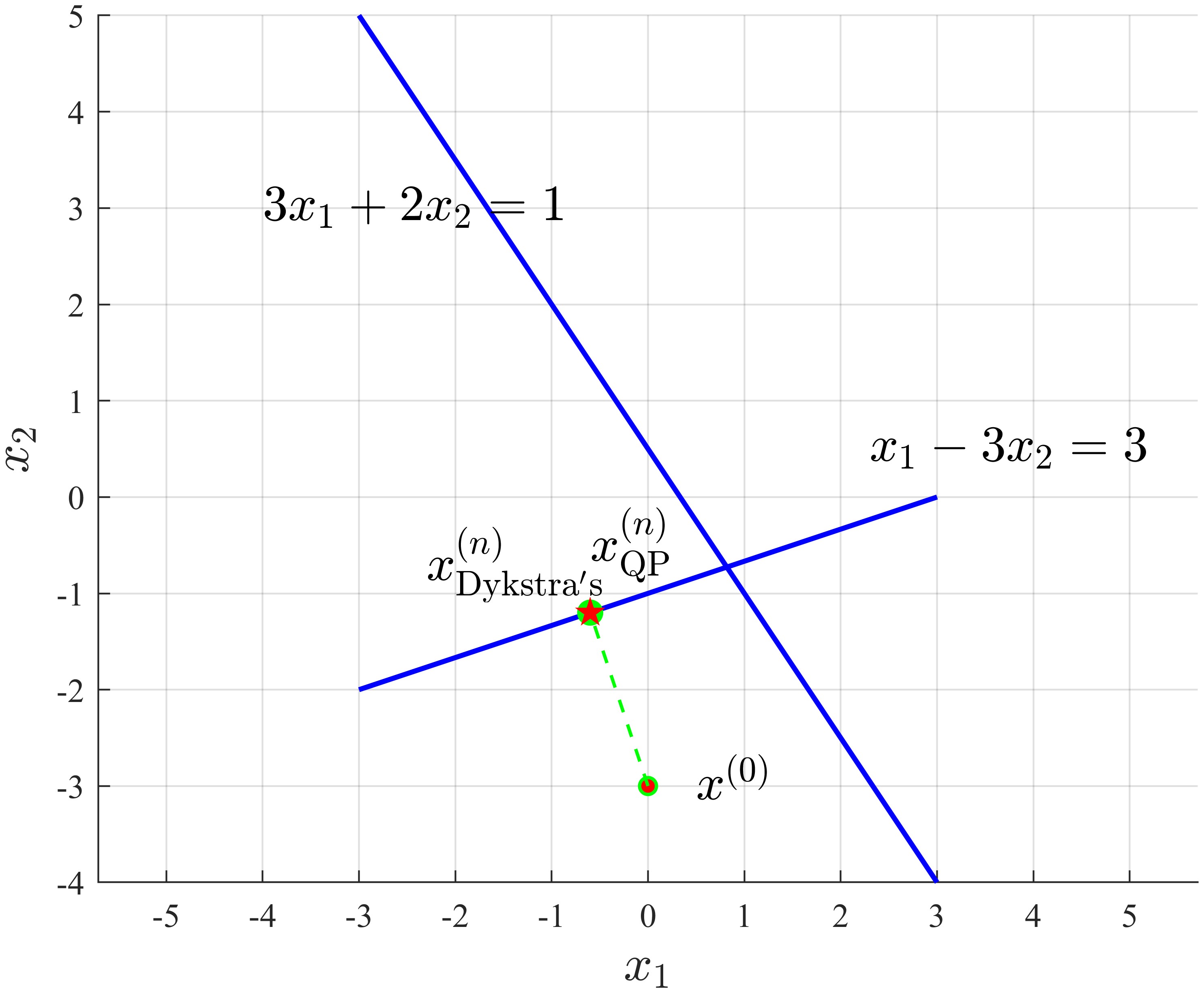
Solution by Dykstra's: (-0.6000, -1.2000)
Solution by solving QP: (-0.6000, -1.2000)
1
2
3
4
5
6
7
8
9
10
11
12
13
14
15
16
17
18
19
20
21
22
23
24
25
26
27
28
29
30
31
32
33
34
35
36
37
38
39
40
41
42
43
44
45
46
47
48
49
50
51
52
53
54
55
56
57
58
59
60
61
62
63
64
65
66
67
68
69
70
71
72
73
74
75
76
77
78
79
80
81
82
clc, clear, close all

x1 = linspace(-3, 3, 200);
a = [3, 1;
    2, -3];
b = [1; 3];

figure('Color', 'w')
hold(gca, 'on')
grid(gca, 'on')
plot(x1, (1-3*x1)/2, 'LineWidth', 1.5, 'Color', 'b', 'HandleVisibility', 'off')
text(-4, 3, '$3x_1+2x_2=1$', 'Interpreter', 'latex', 'FontSize', 15)
plot(x1, (1/3)*x1-1, 'LineWidth', 1.5, 'Color', 'b', 'HandleVisibility', 'off')
text(2.3, 0.5, '$x_1-3x_2=3$', 'Interpreter', 'latex', 'FontSize', 15)
axis('equal')

x0 = [0; -3];
scatter(x0(1), x0(2), 30, 'filled', 'MarkerFaceColor', 'r', 'HandleVisibility', 'off')
text(x0(1)+0.5, x0(2), '$x^{(0)}$', 'Interpreter', 'latex', 'FontSize', 15)

numVariables = 2;
d = 2; % Num of constraints
numEpoch = 1e3;

% Num of variables * num of constraints * iterations
u = nan(numVariables, d+1, numEpoch+1); % points after projection
z = zeros(numVariables, d, numEpoch+1); % auxiliar variables

for i = 0:d
    u(:, i+1, 1) = x0;
end

for k = 2:numEpoch
    u(:, 1, k) = u(:, d+1, k-1);

    for i = 1:d
        uiOld = u(:, i,   k);
        ziOld = z(:, i,   k-1);
        u(:, i+1, k) = helperProjec(a(:,i), b(i), (uiOld+ziOld));
        z(:, i, k) = uiOld + ziOld - u(:, i+1, k);
    end

    if norm(u(:, d+1, k) - u(:, d+1, k-1)) < 1e-4
        break;
    end
end

u(:, :, k+1:end) = [];
z(:, :, k+1:end) = [];

for i = 1:size(u,3)-1
    plot([u(1,d+1,i), u(1,d+1,i+1)], [u(2,d+1,i), u(2,d+1,i+1)], ...
        'LineWidth', 1, 'Color', 'g', 'LineStyle', '--', ...
        'Marker', 'o', 'MarkerSize', 5,...
        'HandleVisibility', 'off')
end

x_projection = u(:,d+1,end);
x_qp = quadprog(eye(2) , -x0, a', b);

scatter(x_projection(1), x_projection(2), 60, 'filled', 'MarkerFaceColor', 'g', 'HandleVisibility', 'off')
text(x_projection(1)-1.7, x_projection(2)+0.5, '$x^{(n)}_\mathrm{Dykstra^\prime s}$', 'Interpreter', 'latex', 'FontSize', 15)
fprintf('Solution by Dykstra''s: (%.4f, %.4f)\n', x_projection(1), x_projection(2))

scatter(x_qp(1), x_qp(2), 90, 'filled', 'Marker', 'pentagram', 'MarkerFaceColor', 'r', 'HandleVisibility', 'off')
text(x_qp(1), x_qp(2)+0.7, '$x^{(n)}_\mathrm{QP}$', 'Interpreter', 'latex', 'FontSize', 15)
fprintf('Solution by solving QP: (%.4f, %.4f)\n', x_qp(1), x_qp(2))

legend('Box', 'off', 'FontSize', 15)
xlabel('$x_1$', 'Interpreter', 'latex', 'FontSize', 15)
ylabel('$x_2$', 'Interpreter', 'latex', 'FontSize', 15)
set(gca, 'FontName', 'Times New Roman')

exportgraphics(gca, 'fig2.jpg', 'Resolution', 600)

function x_pc = helperProjec(a, b, x0)
if a'*x0<=b
    x_pc = x0;
else
    x_pc = x0+(b-a'*x0)*a/norm(a)^2;
end
end
Three-set example
1
2
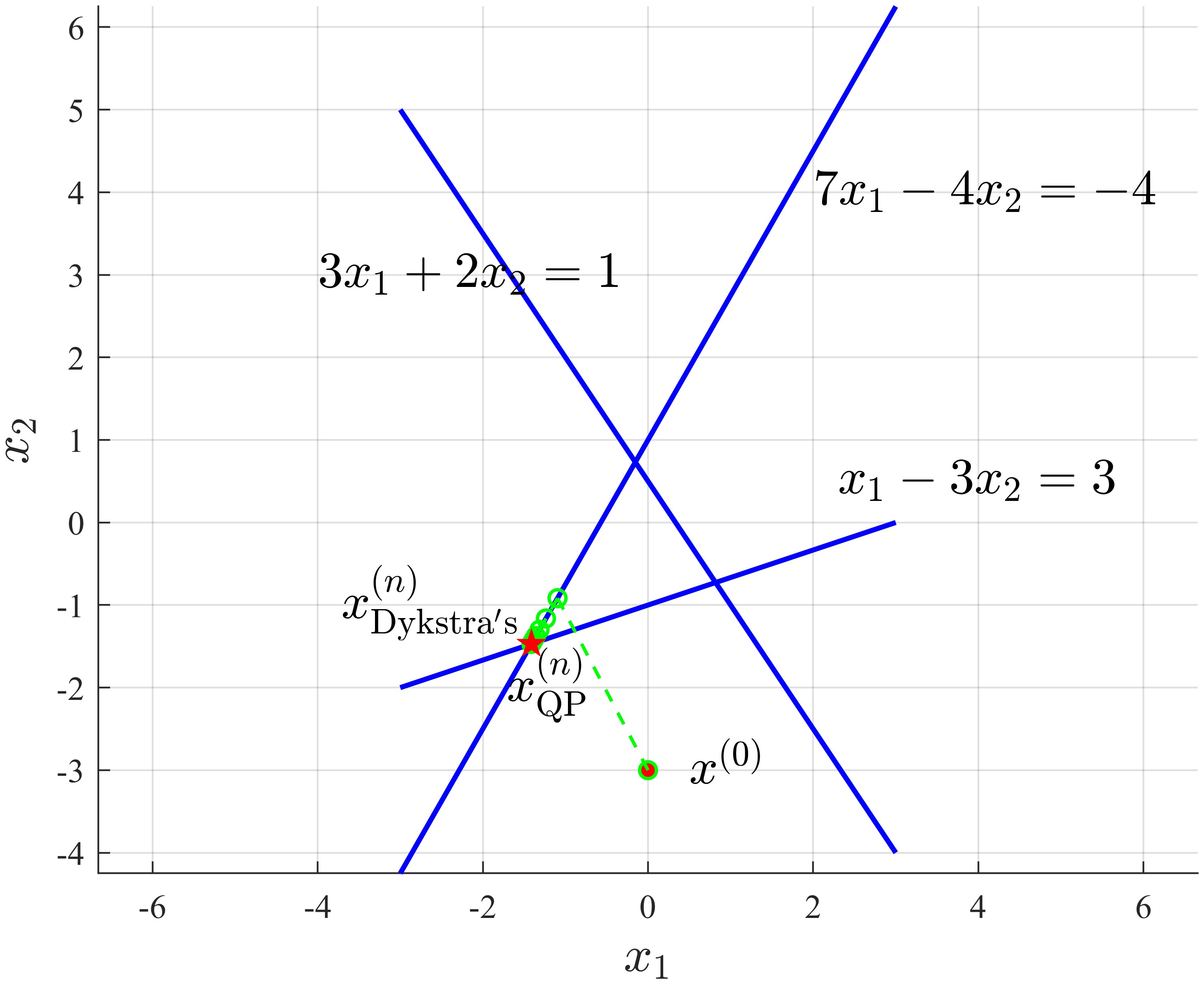
Solution by Dykstra's: (-1.4117, -1.4705)
Solution by solving QP: (-1.4118, -1.4706)
Right now, we can easily see the difference between the results of POCS and Dykstra’s projection algorithm — again, Dykstra’s projection algorithm finds a feasible point whose distance from $\boldsymbol{x}^{(0)}$ is the least, the same as QP’s solution; POCS only find “some point” that is feasible.
1
2
3
4
5
6
7
8
9
10
11
12
13
14
15
16
17
18
19
20
21
22
23
24
25
26
27
28
29
30
31
32
33
34
35
36
37
38
39
40
41
42
43
44
45
46
47
48
49
50
51
52
53
54
55
56
57
58
59
60
61
62
63
64
65
66
67
68
69
70
71
72
73
74
75
76
77
78
79
80
81
82
83
84
clc, clear, close all

x1 = linspace(-3, 3, 200);
a = [3, 1, 7;
    2, -3, -4];
b = [1; 3; -4];

figure('Color', 'w')
hold(gca, 'on')
grid(gca, 'on')
plot(x1, (1-3*x1)/2, 'LineWidth', 1.5, 'Color', 'b', 'HandleVisibility', 'off')
text(-4, 3, '$3x_1+2x_2=1$', 'Interpreter', 'latex', 'FontSize', 15)
plot(x1, (1/3)*x1-1, 'LineWidth', 1.5, 'Color', 'b', 'HandleVisibility', 'off')
text(2.3, 0.5, '$x_1-3x_2=3$', 'Interpreter', 'latex', 'FontSize', 15)
plot(x1, x1/(4/7)+1, 'LineWidth', 1.5, 'Color', 'b', 'HandleVisibility', 'off')
text(2, 4, '$7x_1-4x_2=-4$', 'Interpreter', 'latex', 'FontSize', 15)
axis('equal')

x0 = [0; -3];
scatter(x0(1), x0(2), 30, 'filled', 'MarkerFaceColor', 'r', 'HandleVisibility', 'off')
text(x0(1)+0.5, x0(2), '$x^{(0)}$', 'Interpreter', 'latex', 'FontSize', 15)

numVariables = 2;
d = 3; % Num of constraints
numEpoch = 1e3;

% Num of variables * num of constraints * iterations
u = nan(numVariables, d+1, numEpoch+1); % points after projection
z = zeros(numVariables, d, numEpoch+1); % auxiliar variables

for i = 0:d
    u(:, i+1, 1) = x0;
end

for k = 2:numEpoch
    u(:, 1, k) = u(:, d+1, k-1);

    for i = 1:d
        ui_old = u(:, i,   k);
        zi_old = z(:, i,   k-1);
        u(:, i+1, k) = helperProjec(a(:,i), b(i), (ui_old+zi_old));
        z(:, i, k) = ui_old + zi_old - u(:, i+1, k);
    end

    if norm(u(:, d+1, k) - u(:, d+1, k-1)) < 1e-4
        break;
    end
end

u(:, :, k+1:end) = [];
z(:, :, k+1:end) = [];

for i = 1:size(u,3)-1
    plot([u(1,d+1,i), u(1,d+1,i+1)], [u(2,d+1,i), u(2,d+1,i+1)], ...
        'LineWidth', 1, 'Color', 'g', 'LineStyle', '--', ...
        'Marker', 'o', 'MarkerSize', 5,...
        'HandleVisibility', 'off')
end

x_projection = u(:,d+1,end);
x_qp = quadprog(eye(2) , -x0, a', b);

scatter(x_projection(1), x_projection(2), 30, 'filled', 'MarkerFaceColor', 'g', 'HandleVisibility', 'off')
text(x_projection(1)-2.3, x_projection(2)+0.5, '$x^{(n)}_\mathrm{Dykstra^\prime s}$', 'Interpreter', 'latex', 'FontSize', 15)
fprintf('Solution by Dykstra''s: (%.4f, %.4f)\n', x_projection(1), x_projection(2))

scatter(x_qp(1), x_qp(2), 90, 'filled', 'Marker', 'pentagram', 'MarkerFaceColor', 'r', 'HandleVisibility', 'off')
text(x_qp(1)-0.3, x_qp(2)-0.5, '$x^{(n)}_\mathrm{QP}$', 'Interpreter', 'latex', 'FontSize', 15)
fprintf('Solution by solving QP: (%.4f, %.4f)\n', x_qp(1), x_qp(2))

legend('Box', 'off', 'FontSize', 15)
xlabel('$x_1$', 'Interpreter', 'latex', 'FontSize', 15)
ylabel('$x_2$', 'Interpreter', 'latex', 'FontSize', 15)
set(gca, 'FontName', 'Times New Roman')

exportgraphics(gca, 'fig3.jpg', 'Resolution', 600)

function x_pc = helperProjec(a, b, x0)
if a'*x0<=b
    x_pc = x0;
else
    x_pc = x0+(b-a'*x0)*a/norm(a)^2;
end
end
References