Euclidean Projection on a Polyhedron (Especially, Hyperplane and Halfspace) and POCS Method (i.e., Projections Onto Convex Sets, a.k.a. Alternating Projection Method)

Nov. 16, 2025 in Buffalo, United States • Updated Nov. 23, 2025

Euclidean projection on a polyhedron

When solving an optimization problem with constraints, in some iterations, the solution of control variables may be outside of feasible domain. So, we should use some methods to pull them back into the feasible domain.

The polyhedron¹ described by some linear inequalities is a kind of very classic feasible domain, and in each iteration, we can use Euclidean projection to make those infeasible intermediate solution feasible. The Euclidean projection on a polyhedron is equivalent to solving a Quadratic Problem (QP)²:

where $\boldsymbol{x}_0$ is the infeasible solution we get in the $t$-th iteration, and $\boldsymbol{x}$ to be solved is the final feasible solution we adopt in $t$-th iteration. So, this optimization problem means “find an $\boldsymbol{x}$ in the feasible domain such that whose distance from $\boldsymbol{x}_0$ is the least” — if $x_0$ has satisfied the feasible domain, then the $\boldsymbol{x}$ is simply $\boldsymbol{x}_0$. Btw, this idea is sort of similar to using Least Square Method to get a least-square solution of an over-determined system.³

Sometimes, solving this QP is very difficult, but luckily, for some special cases, we have analytical solutions²:

(1) Projection on a hyperplane⁴

(2) Projection on halfspace⁵

More generally, a half-space is either of the two parts into which a hyperplane divides an n-dimensional space. That is, the points that are not incident to the hyperplane are partitioned into two convex sets (i.e., half-spaces), such that any subspace connecting a point in one set to a point in the other must intersect the hyperplane.

(3) Projection on rectangle

The rectangle case is pretty easy to understand; for hyperplane and halfspace, there is a same formular:

\[P_C(\boldsymbol{x}_0) = \boldsymbol{x}_0+(b-\boldsymbol{a}^T\boldsymbol{x}_0)\boldsymbol{a}/||\boldsymbol{a}||^2_{_2}\label{eq5}\]

Next, I will talk about it.

Projection on a hyperplane

When the feasible domain is a hyperplane, the QP will become:

\[\begin{split} \min_\boldsymbol{x}\,& \frac12||\boldsymbol{x}-\boldsymbol{x}_0||^2_{_2}\\ \text{s.t.}\,& \boldsymbol{a}^T\boldsymbol{x}=b \end{split}\label{eq6}\]

Note, because the feasible domain is a hyperplane, there is only one constraint.

The Lagrangian function for QP $\eqref{eq6}$ is:

\[\begin{split} \mathcal{L}(\boldsymbol{x},\lambda) &= \frac12||\boldsymbol{x}-\boldsymbol{x}_0||^2_{_2}+\lambda(\boldsymbol{a}^T\boldsymbol{x}-b)\\ &=\frac12(\boldsymbol{x}-\boldsymbol{x}_0)^T(\boldsymbol{x}-\boldsymbol{x}_0)+\lambda(\boldsymbol{a}^T\boldsymbol{x}-b) \end{split}\]

so we have:

\[\dfrac{\partial\mathcal{L}}{\partial\boldsymbol{x}}=\boldsymbol{0} \quad\Rightarrow\quad (\boldsymbol{x}-\boldsymbol{x}_0)+\lambda\boldsymbol{a} = \boldsymbol{0}\quad\Rightarrow\quad\boldsymbol{x} = \boldsymbol{x}_0-\lambda\boldsymbol{a}\label{eq1}\] \[\dfrac{\partial\mathcal{L}}{\partial\lambda}=0\quad\Rightarrow\quad\boldsymbol{a}^T\boldsymbol{x}-b=0\quad\Rightarrow\quad\boldsymbol{a}^T\boldsymbol{x} = b\label{eq2}\]

Bring Eq. $\eqref{eq1}$ into Eq. $\eqref{eq2}$, then:

\[\begin{split} \,&\boldsymbol{a}^T(\boldsymbol{x}_0-\lambda\boldsymbol{a}) = b\\ \Rightarrow\,&\boldsymbol{a}^T\boldsymbol{x}_0-\lambda||\boldsymbol{a}||^2_{_2}=b\\ \Rightarrow\,&\lambda=\dfrac{\boldsymbol{a}^T\boldsymbol{x}_0-b}{||\boldsymbol{a}||^2_{_2}} \end{split}\label{eq3}\]

then, again, bring Eq. $\eqref{eq3}$ into $\eqref{eq1}$, so we have:

\[\boldsymbol{x} = \boldsymbol{x}_0-\dfrac{\boldsymbol{a}^T\boldsymbol{x}_0-b}{||\boldsymbol{a}||^2_{_2}}\boldsymbol{a}\]

i.e.,

\[\boldsymbol{x} = \boldsymbol{x}_0+(b-\boldsymbol{a}^T\boldsymbol{x}_0)\boldsymbol{a}/||\boldsymbol{a}||^2_{_2}\label{eq4}\]

that is, Eq. $\eqref{eq5}$.

In Eq. $\eqref{eq4}$, we can get:

$\boldsymbol{a}$ is the normal vector of $\boldsymbol{a}^T\boldsymbol{x}=b$. We can understand this point from two perspectives:
1. $\boldsymbol{a}^T\boldsymbol{x} = b$ is a level set of $g(\boldsymbol{x})=\boldsymbol{a}^T\boldsymbol{x}$, and because the gradient $\nabla g(\boldsymbol{x})$ is orthogonal with tangent of the level set⁶, we can get that $\nabla g(\boldsymbol{x})=\boldsymbol{a}$ is the normal vector of hyperplane $\boldsymbol{a}^T\boldsymbol{x}=b$;
2. Select two (any) points $x_1$ and $x_2$ on the hyperplane $\boldsymbol{a}^T\boldsymbol{x}=b$, i.e., $\boldsymbol{a}^T\boldsymbol{x}_1=b$, $\boldsymbol{a}^T\boldsymbol{x}_2=b$, then we have: $\boldsymbol{a}^T(\boldsymbol{x}_1-\boldsymbol{x}_2)=0$, where $(\boldsymbol{x}_1-\boldsymbol{x}_2)$ is actually a tangent line of $\boldsymbol{a}^T\boldsymbol{x}=b$, so $\boldsymbol{a}$ is the norm vector.
hence, vector $\boldsymbol{a}/\vert\vert\boldsymbol{a}\vert\vert^2_{_2}$ is a vector with the same direction with $\boldsymbol{a}$ (note, $\boldsymbol{a}/\vert\vert\boldsymbol{a}\vert\vert^2_{_2}$ is not a unit vector; the unit vector is $\boldsymbol{a}/\vert\vert\boldsymbol{a}\vert\vert_{_2}$ — tell the difference between the denominator of both), i.e., vector $\boldsymbol{a}/\vert\vert\boldsymbol{a}\vert\vert^2_{_2}$ is perpendicular to hyperplane $\boldsymbol{a}^T\boldsymbol{x}=b$ as well.

So, Eq. $\eqref{eq4}$ means that, we start from $\boldsymbol{x}_0$, along with the direction that is perpendicular to hyperplane $\boldsymbol{a}^T\boldsymbol{x}=b$, until we touch the hyperplane, then the end point that intersects with $\boldsymbol{a}^T\boldsymbol{x}=b$ is the solution we expect, $\boldsymbol{x}$.

The new vector $\boldsymbol{x}$ must be on the hyperplane $\boldsymbol{a}^T\boldsymbol{x}=b$, because: (1) on the one hand, we derived $\eqref{eq4}$ using Lagrange method as above, so $\boldsymbol{x}$ must be in the feasible domain, and (2) on the other hand, we can simply verify it by:

\[\begin{split} \boldsymbol{a}^T\boldsymbol{x} &= \boldsymbol{a}^T(\boldsymbol{x}_0+(b-\boldsymbol{a}^T\boldsymbol{x}_0)\boldsymbol{a}/||\boldsymbol{a}||^2_{_2})\\ &= \boldsymbol{a}^T\boldsymbol{x}_0+(b-\boldsymbol{a}^T\boldsymbol{x}_0)\\ &= b \end{split}\]

Projection on a halfspace

After explaining the hyperplane case, then at this time, we can easily understand the projection on the halfspace is:

\[P_C(\boldsymbol{x}) = \left\{\begin{split} &\boldsymbol{x}_0+(b-\boldsymbol{a}^T\boldsymbol{x}_0)\boldsymbol{a}/||\boldsymbol{a}||^2_{_2}\quad&\boldsymbol{a}^T\boldsymbol{x}_0>b\\ &\boldsymbol{x}_0\quad&\boldsymbol{a}^T\boldsymbol{x}_0\le b\\ \end{split}\right.\label{eq7}\]

POCS method (a.k.a. Alternating projection method)

In the following content, I’ll test some examples.

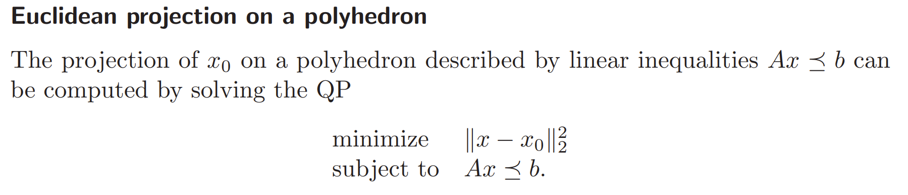
Halfspace example

Consider the halfspace:

\[3x_1+2x_2\le1\]

(where $\boldsymbol{a} = [3,2]^T$ and $b=1$) and $\boldsymbol{x}_0 = [4,-2]^T$, then we can conduct Euclidean projection in MATLAB as below:

clc, clear, close all

x1 = linspace(-3, 3, 200);
a = [3; 2];
b = 1;

figure('Color', 'w')
hold(gca, 'on')
plot(x1, (1-3*x1)/2, 'LineWidth', 1.5, 'Color', 'b', 'HandleVisibility', 'off')
text(-4, 3, '$3x_1+2x_2=1$', 'Interpreter', 'latex', 'FontSize', 15)
axis('equal')

x0 = [4; -2];
scatter(x0(1), x0(2), 30, 'filled', 'MarkerFaceColor', 'r', 'HandleVisibility', 'off')
text(x0(1)+0.5, x0(2), '$x^{(0)}$', 'Interpreter', 'latex', 'FontSize', 15)

x_Pc = helperProjec(a, b, x0);
scatter(x_Pc(1), x_Pc(2), 30, 'filled', 'MarkerFaceColor', 'b', 'HandleVisibility', 'off')
text(x_Pc(1)+0.5, x_Pc(2), '$x^{(1)}$', 'Interpreter', 'latex', 'FontSize', 15)
plot([x0(1), x_Pc(1)], [x0(2), x_Pc(2)], ...
    'LineWidth', 1.5, 'Color', 'r', 'LineStyle', '--', 'DisplayName', '1st Projection')


legend('Box', 'off', 'FontSize', 15)
xlabel('$x_1$', 'Interpreter', 'latex', 'FontSize', 15)
ylabel('$x_2$', 'Interpreter', 'latex', 'FontSize', 15)
set(gca, 'FontName', 'Times New Roman')

exportgraphics(gca, 'fig1.jpg', 'Resolution', 600)

function x_pc = helperProjec(a, b, x0)
if a'*x0<=b
    x_pc = x0;
else
    x_pc = x0+(b-a'*x0)*a/norm(a)^2;
end
end

fig1

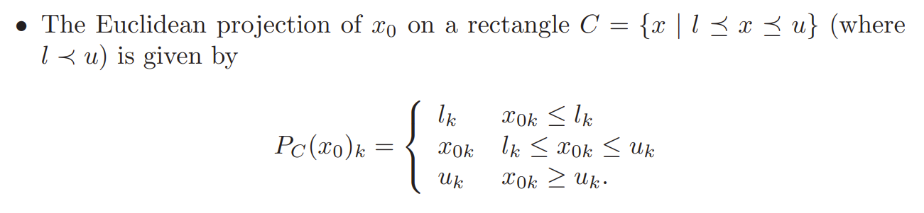
Polyhedron examples

Consider a polyhedron:

\[\begin{split} &3x_1+2x_2\le1\\ &x_1-x_2\le1 \end{split}\label{eq9}\]

which can be written as matrix form:

\[\begin{bmatrix} 3 & 2\\ 1 & -1\\ \end{bmatrix} \begin{bmatrix} x_1\\x_2 \end{bmatrix} \preceq \begin{bmatrix} 1\\ 1 \end{bmatrix}\]

It should highlight that, $\eqref{eq9}$ is a polyhedron, NOT a halfspace (in fact, it is a polyhedron described by two halfspaces). So, using Eq. $\eqref{eq7}$ doesn’t guarantee we can get a minimum of the QP. But we can still have a try.

If we also want to use Eq. $\eqref{eq7}$, a natural idea is to consider (i.e., conduct projection on) each halfspace one by one:

clc, clear, close all

x1 = linspace(-3, 3, 200);
a = [3, 1;
    2, -1];
b = [1; 1];

figure('Color', 'w')
hold(gca, 'on')
grid(gca, 'on')
plot(x1, (1-3*x1)/2, 'LineWidth', 1.5, 'Color', 'b', 'HandleVisibility', 'off')
text(-4, 3, '$3x_1+2x_2=1$', 'Interpreter', 'latex', 'FontSize', 15)
plot(x1, x1-1, 'LineWidth', 1.5, 'Color', 'b', 'HandleVisibility', 'off')
text(2.3, 1, '$x_1-x_2=1$', 'Interpreter', 'latex', 'FontSize', 15)
axis('equal')

x0 = [4; -2];
scatter(x0(1), x0(2), 30, 'filled', 'MarkerFaceColor', 'r', 'HandleVisibility', 'off')
text(x0(1)+0.5, x0(2), '$x^{(0)}$', 'Interpreter', 'latex', 'FontSize', 15)

x_Pc1 = helperProjec(a(:,1), b(1), x0);
scatter(x_Pc1(1), x_Pc1(2), 30, 'filled', 'MarkerFaceColor', 'b', 'HandleVisibility', 'off')
plot([x0(1), x_Pc1(1)], [x0(2), x_Pc1(2)], ...
    'LineWidth', 1.5, 'Color', 'r', 'LineStyle', '--', 'DisplayName', '1st Projection')
text(x_Pc1(1)+0.5, x_Pc1(2), '$x^{(1)}$', 'Interpreter', 'latex', 'FontSize', 15)

x_Pc2 = helperProjec(a(:,2), b(2), x_Pc1);
scatter(x_Pc2(1), x_Pc2(2), 30, 'filled', 'MarkerFaceColor', 'g', 'HandleVisibility', 'off')
plot([x_Pc1(1), x_Pc2(1)], [x_Pc1(2), x_Pc2(2)], ...
    'LineWidth', 1.5, 'Color', 'g', 'LineStyle', '--', 'DisplayName', '2nd Projection')
text(x_Pc2(1)-1, x_Pc2(2), '$x^{(2)}$', 'Interpreter', 'latex', 'FontSize', 15)

legend('Box', 'off', 'FontSize', 15)
xlabel('$x_1$', 'Interpreter', 'latex', 'FontSize', 15)
ylabel('$x_2$', 'Interpreter', 'latex', 'FontSize', 15)
set(gca, 'FontName', 'Times New Roman')

exportgraphics(gca, 'fig2.jpg', 'Resolution', 600)

function x_pc = helperProjec(a, b, x0)
if a'*x0<=b
    x_pc = x0;
else
    x_pc = x0+(b-a'*x0)*a/norm(a)^2;
end
end

fig2

Luckily, this method works: after two projection, we got a solution in the feasible domain.

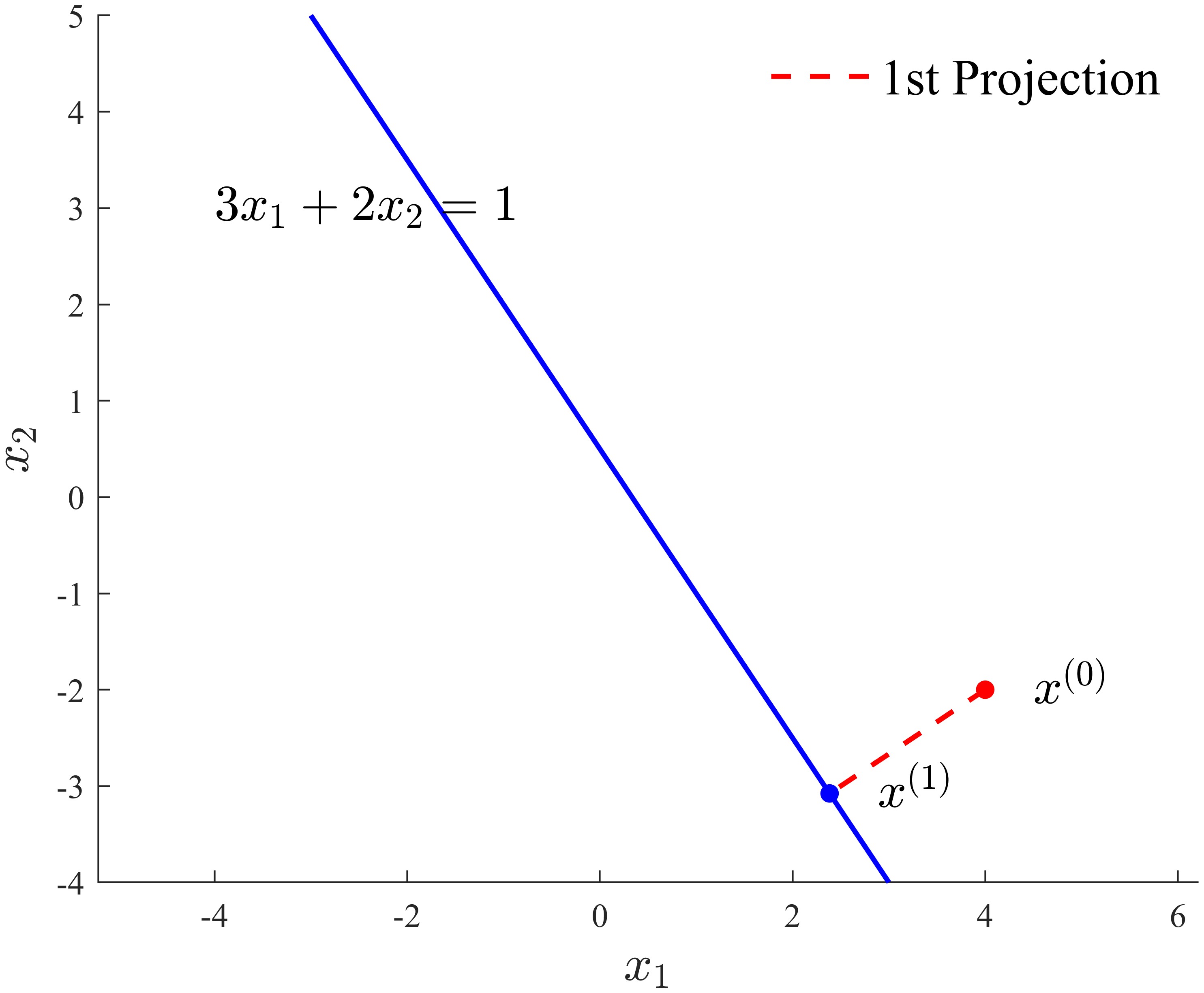
However, if we change the second halfspace as $x_1-3x_2\le3$, i.e.,

\[\begin{split} &3x_1+2x_2\le1\\ &x_1-3x_2\le3 \end{split}\label{eq10}\]

and still use $\boldsymbol{x}_0 = [4,-2]^T$, then we have:

clc, clear, close all

x1 = linspace(-3, 3, 200);
a = [3, 1;
    2, -3];
b = [1; 3];

figure('Color', 'w')
hold(gca, 'on')
grid(gca, 'on')
plot(x1, (1-3*x1)/2, 'LineWidth', 1.5, 'Color', 'b', 'HandleVisibility', 'off')
text(-4, 3, '$3x_1+2x_2=1$', 'Interpreter', 'latex', 'FontSize', 15)
plot(x1, (1/3)*x1-1, 'LineWidth', 1.5, 'Color', 'b', 'HandleVisibility', 'off')
text(2.3, 0.5, '$x_1-3x_2=3$', 'Interpreter', 'latex', 'FontSize', 15)
axis('equal')

x0 = [4; -2];
scatter(x0(1), x0(2), 30, 'filled', 'MarkerFaceColor', 'r', 'HandleVisibility', 'off')
text(x0(1)+0.5, x0(2), '$x^{(0)}$', 'Interpreter', 'latex', 'FontSize', 15)

x_Pc1 = helperProjec(a(:,1), b(1), x0);
scatter(x_Pc1(1), x_Pc1(2), 30, 'filled', 'MarkerFaceColor', 'b', 'HandleVisibility', 'off')
plot([x0(1), x_Pc1(1)], [x0(2), x_Pc1(2)], ...
    'LineWidth', 1.5, 'Color', 'r', 'LineStyle', '--', 'DisplayName', '1st Projection')
text(x_Pc1(1)+0.5, x_Pc1(2), '$x^{(1)}$', 'Interpreter', 'latex', 'FontSize', 15)

x_Pc2 = helperProjec(a(:,2), b(2), x_Pc1);
scatter(x_Pc2(1), x_Pc2(2), 30, 'filled', 'MarkerFaceColor', 'g', 'HandleVisibility', 'off')
plot([x_Pc1(1), x_Pc2(1)], [x_Pc1(2), x_Pc2(2)], ...
    'LineWidth', 1.5, 'Color', 'g', 'LineStyle', '--', 'DisplayName', '2nd Projection')
text(x_Pc2(1)+0.5, x_Pc2(2), '$x^{(2)}$', 'Interpreter', 'latex', 'FontSize', 15)

legend('Box', 'off', 'FontSize', 15)
xlabel('$x_1$', 'Interpreter', 'latex', 'FontSize', 15)
ylabel('$x_2$', 'Interpreter', 'latex', 'FontSize', 15)
set(gca, 'FontName', 'Times New Roman')

exportgraphics(gca, 'fig3.jpg', 'Resolution', 600)

function x_pc = helperProjec(a, b, x0)
if a'*x0<=b
    x_pc = x0;
else
    x_pc = x0+(b-a'*x0)*a/norm(a)^2;
end
end

fig3

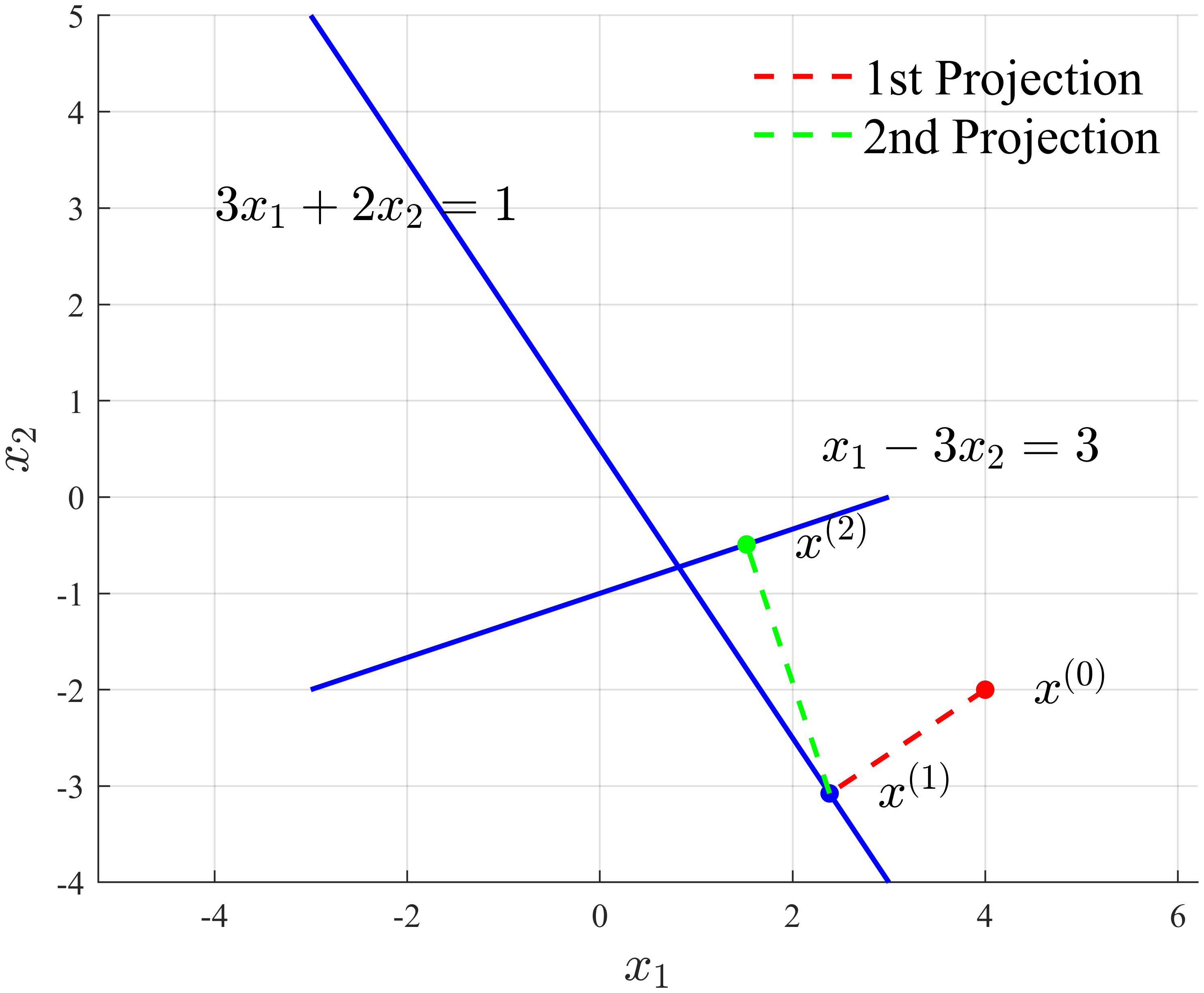
So, at this time, the final point isn’t in the feasible domain.

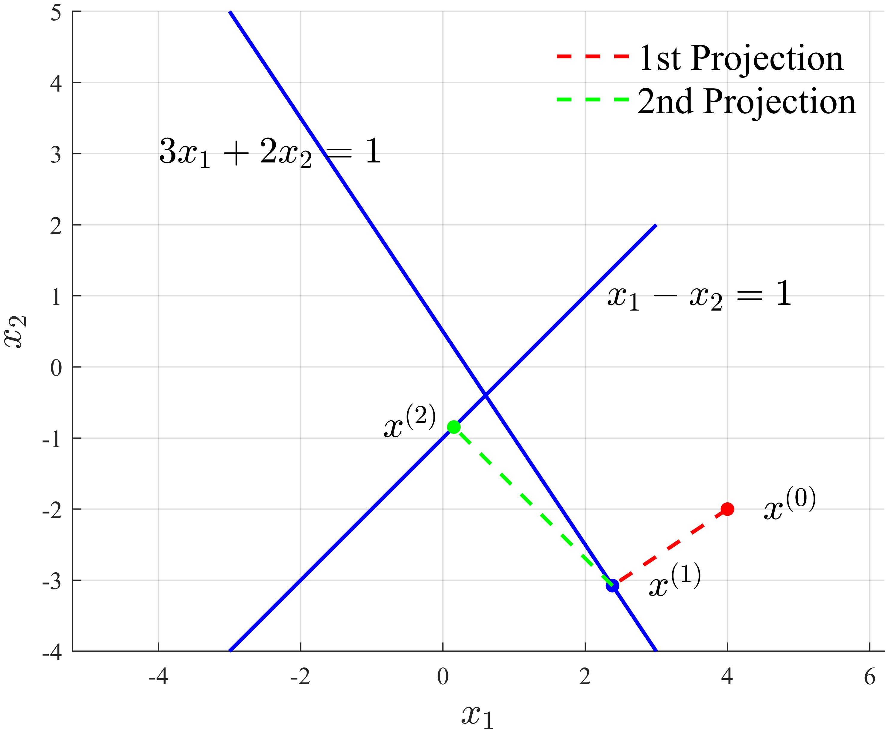
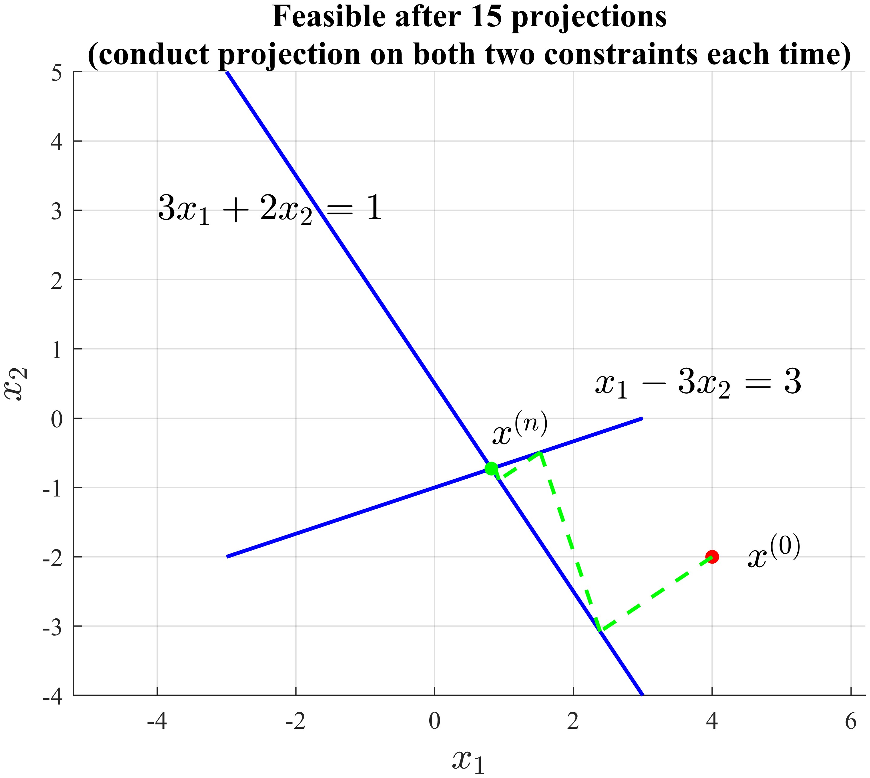
POCS method

However, above result can inspire us to continue conducting projection on $3x_1+2x_2=1$ and then $x_1-3x_2=3$, again and again, until both constraints are satisfied. We can use a while loop to realize this point:

clc, clear, close all

x1 = linspace(-3, 3, 200);
a = [3, 1;
    2, -3];
b = [1; 3];

figure('Color', 'w')
hold(gca, 'on')
grid(gca, 'on')
plot(x1, (1-3*x1)/2, 'LineWidth', 1.5, 'Color', 'b', 'HandleVisibility', 'off')
text(-4, 3, '$3x_1+2x_2=1$', 'Interpreter', 'latex', 'FontSize', 15)
plot(x1, (1/3)*x1-1, 'LineWidth', 1.5, 'Color', 'b', 'HandleVisibility', 'off')
text(2.3, 0.5, '$x_1-3x_2=3$', 'Interpreter', 'latex', 'FontSize', 15)
axis('equal')

x0 = [4; -2];
scatter(x0(1), x0(2), 30, 'filled', 'MarkerFaceColor', 'r', 'HandleVisibility', 'off')
text(x0(1)+0.5, x0(2), '$x^{(0)}$', 'Interpreter', 'latex', 'FontSize', 15)

ntimes = 0;
while ~all(a'*x0 <= b)
    x_Pc1 = helperProjec(a(:,1), b(1), x0);
    plot([x0(1), x_Pc1(1)], [x0(2), x_Pc1(2)], 'LineWidth', 1.5, 'Color', 'g', 'LineStyle', '--', 'HandleVisibility', 'off')

    x_Pc2 = helperProjec(a(:,2), b(2), x_Pc1);
    plot([x_Pc1(1), x_Pc2(1)], [x_Pc1(2), x_Pc2(2)], 'LineWidth', 1.5, 'Color', 'g', 'LineStyle', '--', 'HandleVisibility', 'off')

    x0 = x_Pc2;

    ntimes = ntimes+1;
end

scatter(x_Pc2(1), x_Pc2(2), 30, 'filled', 'MarkerFaceColor', 'g', 'HandleVisibility', 'off')
text(x_Pc2(1), x_Pc2(2)+0.5, '$x^{(n)}$', 'Interpreter', 'latex', 'FontSize', 15)

legend('Box', 'off', 'FontSize', 15)
xlabel('$x_1$', 'Interpreter', 'latex', 'FontSize', 15)
ylabel('$x_2$', 'Interpreter', 'latex', 'FontSize', 15)
set(gca, 'FontName', 'Times New Roman')
title(sprintf(['Feasible after %d projections\n' ...
    '(conduct projection on both two constraints each time)'], ntimes), 'FontSize', 13)

exportgraphics(gca, 'fig4.jpg', 'Resolution', 600)

function x_pc = helperProjec(a, b, x0)
if a'*x0<=b
    x_pc = x0;
else
    x_pc = x0+(b-a'*x0)*a/norm(a)^2;
end
end

fig4

And we can zoom in to look at some details:

fig5

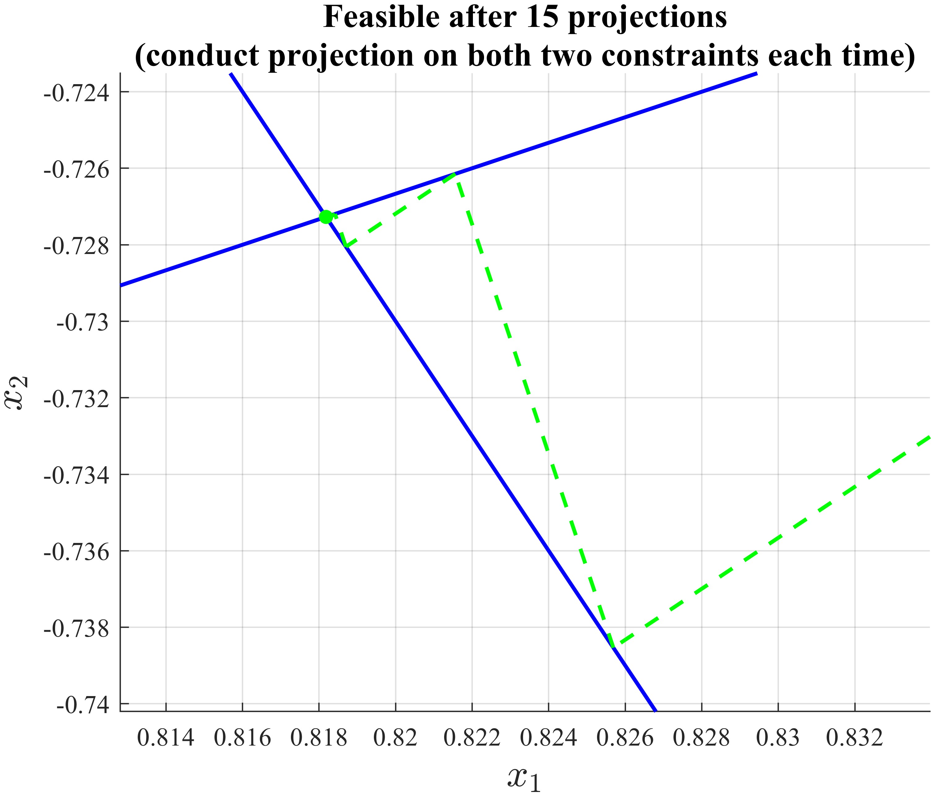
where the final solution is $(0.8182,-0.7273)$.

Actually, this is the basic idea of POCS (projections onto convex sets) algorithm, a.k.a. alternating projection method⁷!!!

Note, any polyhedron is convex⁸.

The POCS algorithm solves the following problem:

\[\text{find}\,\boldsymbol{x}\in\mathbb{R}^n\quad \text{such that}\,\boldsymbol{x}\in C\cap D\]

where $C$ and $D$ are closed⁹ convex sets.

To use the POCS algorithm, one must know how to project onto the sets $C$ and $D$ separately, via the projections $\mathcal{P}_i$.

The algorithm starts with an arbitrary value for $\boldsymbol{x}_0$ and then generates the sequence:

\[\boldsymbol{x}_{k+1} = \mathcal{P}_C(\mathcal{P}_D(\boldsymbol{x}_k))\]

The simplicity of the algorithm explains some of its popularity. If the intersection of $C$ and $D$ is non-empty, then the sequence generated by the algorithm will converge to some point in this intersection.

Projections_onto_convex_sets_circles

Interesting!

By the way, for polyhedron $\eqref{eq10}$, we can write the complete QP of it:

\[\begin{split} \min_\boldsymbol{x}\,&\frac12||\boldsymbol{x}-\boldsymbol{x}_0||^2_{_2}\\ \text{s.t.} \,&\begin{bmatrix} 3 & 2 \\ 1 & -3\\ \end{bmatrix} \begin{bmatrix} x_1 \\ x_2 \end{bmatrix} \preceq \begin{bmatrix} 1 \\ 3 \end{bmatrix} \end{split}\]

re-write it as a standard form:

\[\begin{split} \min_\boldsymbol{x}\,&\dfrac12\boldsymbol{x}^T\boldsymbol{x}-\boldsymbol{x}_0^T\boldsymbol{x}+\dfrac12\boldsymbol{x}_0^T\boldsymbol{x}_0\\ \text{s.t.} \,&\begin{bmatrix} 3 & 2 \\ 1 & -3\\ \end{bmatrix} \begin{bmatrix} x_1 \\ x_2 \end{bmatrix} \preceq \begin{bmatrix} 1 \\ 3 \end{bmatrix} \end{split}\]

then, we can directly use MATLAB quadprog function¹⁰ to solve this QP and look at the result:

clc, clear, close all

x1 = linspace(-3, 3, 200);
a = [3, 1;
    2, -3];
b = [1; 3];

figure('Color', 'w')
hold(gca, 'on')
grid(gca, 'on')
plot(x1, (1-3*x1)/2, 'LineWidth', 1.5, 'Color', 'b', 'HandleVisibility', 'off')
text(-4, 3, '$3x_1+2x_2=1$', 'Interpreter', 'latex', 'FontSize', 15)
plot(x1, (1/3)*x1-1, 'LineWidth', 1.5, 'Color', 'b', 'HandleVisibility', 'off')
text(2.3, 0.5, '$x_1-3x_2=3$', 'Interpreter', 'latex', 'FontSize', 15)
axis('equal')

x0 = [4; -2];
scatter(x0(1), x0(2), 30, 'filled', 'MarkerFaceColor', 'r', 'HandleVisibility', 'off')
text(x0(1)+0.5, x0(2), '$x^{(0)}$', 'Interpreter', 'latex', 'FontSize', 15)

x = quadprog(eye(2) , -x0, a', b);

scatter(x(1), x(2), 30, 'filled', 'MarkerFaceColor', 'g', 'HandleVisibility', 'off')
text(x(1), x(2)+0.5, '$x^{(n)}$', 'Interpreter', 'latex', 'FontSize', 15)

legend('Box', 'off', 'FontSize', 15)
xlabel('$x_1$', 'Interpreter', 'latex', 'FontSize', 15)
ylabel('$x_2$', 'Interpreter', 'latex', 'FontSize', 15)
set(gca, 'FontName', 'Times New Roman')

exportgraphics(gca, 'fig6.jpg', 'Resolution', 600)

fig6

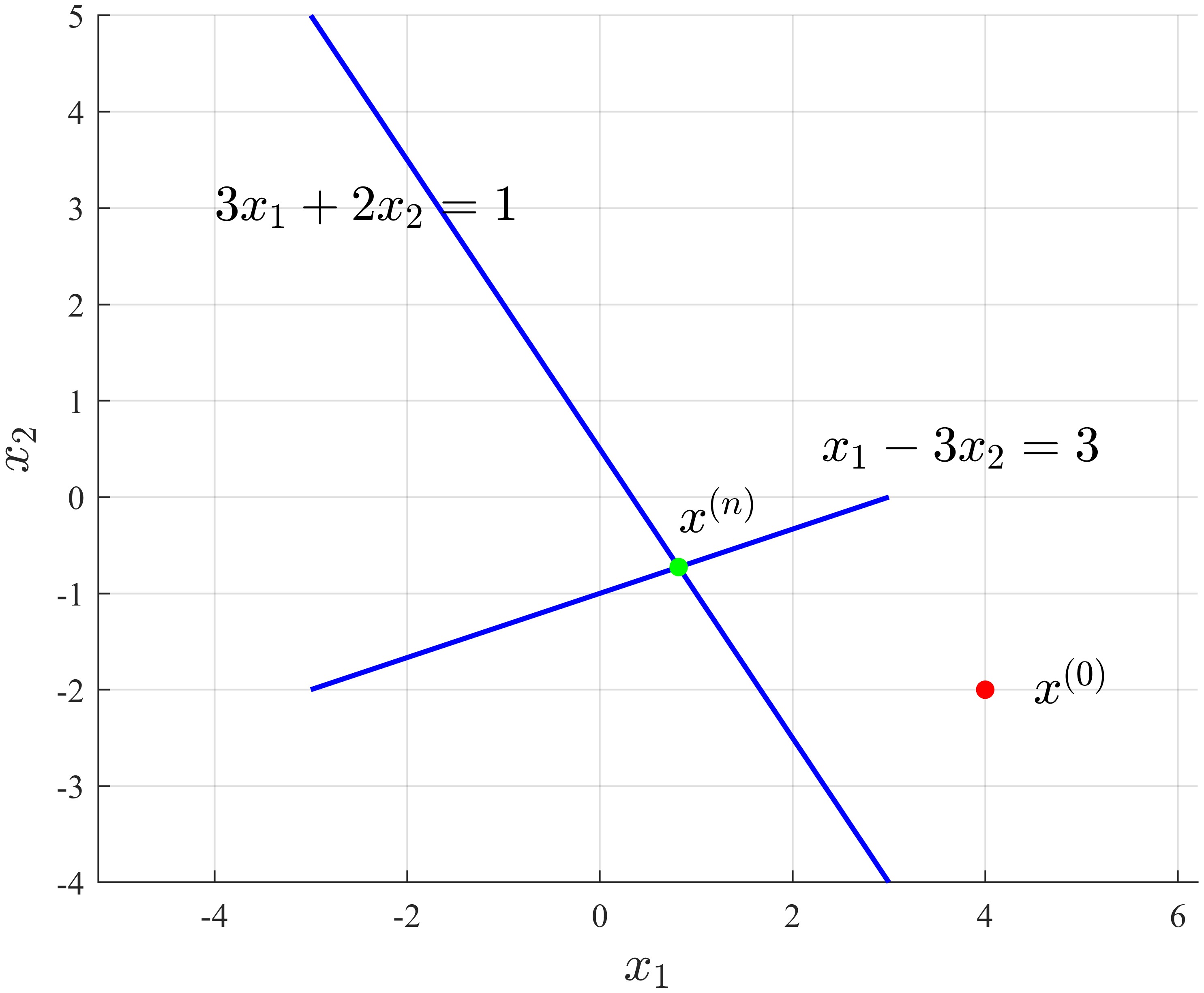
As can be seen, we’ll get the same solution.

POCS vs. Dykstra’s projection algorithm

However, it should be noted that, POCS can only find a point in the feasible domain (polyhedron in above cases), it can’t guarantee the point is the one whose distance from initial value is the least, or rather, it can’t guarantee the point is the solution of corresponding QP. At this time, we need to use Dykstra’s projection algorithm. Please see my another blog¹¹.

References