Introduction

MATLAB provides an example, “View Network Behavior Using tsne”¹, showing how to use t-distributed Stochastic Neighbor Embedding (t-SNE)²³⁴ technique, which is a nonlinear dimension reduction algorithm, to analyze activations of neural network layers.

“This technique (t-SNE) maps high-dimensional data (such as network activations in a layer) to two dimensions. The technique uses a nonlinear map that attempts to preserve distances. By using t-SNE to visualize the network activations, you can gain an understanding of how the network responds.”

“You can use t-SNE to visualize how deep learning networks change the representation of input data as it passes through the network layers. You can also use t-SNE to find issues with the input data and to understand which observations the network classifies incorrectly.”

“For example, t-SNE can reduce the multidimensional activations of a softmax layer to a 2-D representation with a similar structure. Tight clusters in the resulting t-SNE plot correspond to classes that the network usually classifies correctly. The visualization allows you to find points that appear in the wrong cluster, indicating an observation that the network classifies incorrectly. The observation might be (1) labeled incorrectly, or (2) the network might predict that an observation is an instance of a different class because it appears similar to other observations from that class. Note that the t-SNE reduction of the softmax activations uses only those activations, not the underlying observations.”

So, I will reproduce this example and take some notes about it in this post.

Download the image dataset

This example uses the “Example Food Images” data set, which contains 978 photographs of food in nine classes, i.e., caesar_salad, caprese_salad, french_fries, greek_salad, hamburger, hot_dog, pizza, sashimi, and sushi. The data set is also provided by MathWorks, and users can download it from url https://www.mathworks.com/supportfiles/nnet/data/ExampleFoodImageDataset.zip by websave function⁵. All of downloading steps are encapsulated in the helper function downloadExampleFoodImagesData, which can be found in the example.

1
2
3
4
5
6
7
8
9
10
11
12
13
14
15
16
17
18
19
20
21
22
23
24
25
26
27
28
29
30
31
32
33
34
35
36
37
38
39
40
41
42
clc,clear,close all

dataDir = fullfile(pwd,"ExampleFoodImageDataset");
url = "https://www.mathworks.com/supportfiles/nnet/data/ExampleFoodImageDataset.zip";

if ~exist(dataDir,"dir")
    mkdir(dataDir);
end

downloadExampleFoodImagesData(url,dataDir);

function downloadExampleFoodImagesData(url,dataDir)
% Download the Example Food Image data set, containing 978 images of
% different types of food split into 9 classes.
% Copyright 2019 The MathWorks, Inc.

fileName = "ExampleFoodImageDataset.zip";
fileFullPath = fullfile(dataDir,fileName);

% Download the .zip file into a temporary directory.
if ~exist(fileFullPath,"file")
    fprintf("Downloading MathWorks Example Food Image dataset...\n");
    fprintf("This can take several minutes to download...\n");
    websave(fileFullPath,url);
    fprintf("Download finished...\n");
else
    fprintf("Skipping download, file already exists...\n");
end

% Unzip the file.
% Check if the file has already been unzipped by checking for the presence
% of one of the class directories.
exampleFolderFullPath = fullfile(dataDir,"pizza");
if ~exist(exampleFolderFullPath, "dir")
    fprintf("Unzipping file...\n");
    unzip(fileFullPath, dataDir);
    fprintf("Unzipping finished...\n");
else
    fprintf("Skipping unzipping, file already unzipped...\n");
end
fprintf("Done.\n");
end

Train and test the neural network

The following script conducts a standard workflow of neural network training and test to realize image classification.

1
2
3
4
5
6
7
8
9
10
11
12
13
14
15
16
17
18
19
20
21
22
23
24
25
26
27
28
29
30
31
32
33
34
35
36
37
38
39
40
41
42
43
44
45
46
47
clc,clear,close all
rng("default")

% Load the dataset
dataDir = fullfile(pwd,"ExampleFoodImageDataset");

% Define network structure
lgraph = layerGraph(squeezenet());
lgraph = lgraph.replaceLayer("ClassificationLayer_predictions",...
    classificationLayer("Name","ClassificationLayer_predictions"));

newConv =  convolution2dLayer([14,14],9,"Name","conv","Padding","same");
lgraph = lgraph.replaceLayer("conv10",newConv);

% Create training and validation dataset
imds = imageDatastore(dataDir, ...
    "IncludeSubfolders",true,"LabelSource","foldernames");
aug = imageDataAugmenter("RandXReflection",true, ...
    "RandYReflection",true, ...
    "RandXScale",[0.8,1.2], ...
    "RandYScale",[0.8,1.2]);

% Dataset partition and augmentation
trainingFraction = 0.65; % Specify training ratio
[trainImds,valImds] = splitEachLabel(imds,trainingFraction);
augImdsTrain = augmentedImageDatastore([227,227],trainImds, ...
    "DataAugmentation",aug);
augImdsVal = augmentedImageDatastore([227,227],valImds);

% Train the network
options = trainingOptions("adam", ...
    "InitialLearnRate",1e-4, ...
    "MaxEpochs",30, ...
    "ValidationData",augImdsVal, ...
    "Verbose",false,...
    "Plots","training-progress", ...
    "ExecutionEnvironment","auto",...
    "MiniBatchSize",128);
net = trainNetwork(augImdsTrain,lgraph,options);

% Test the network
figure("Color","w");
YPred = classify(net,augImdsVal);
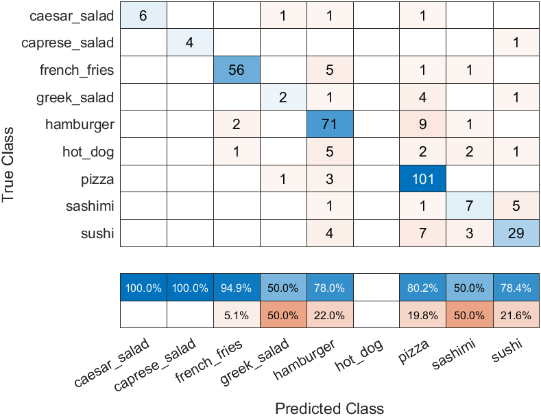
confusionchart(valImds.Labels,YPred,"ColumnSummary","column-normalized")

save("results.mat", ...
    "trainImds","valImds","augImdsTrain","augImdsVal","net","YPred")

The corresponding training process is:

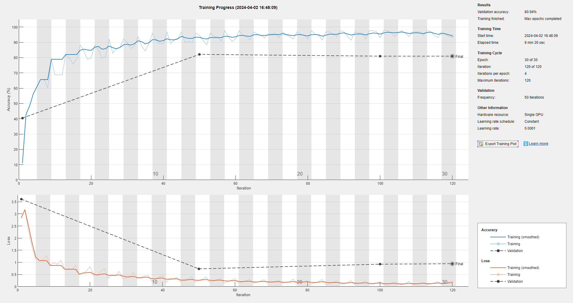
and the test result is:

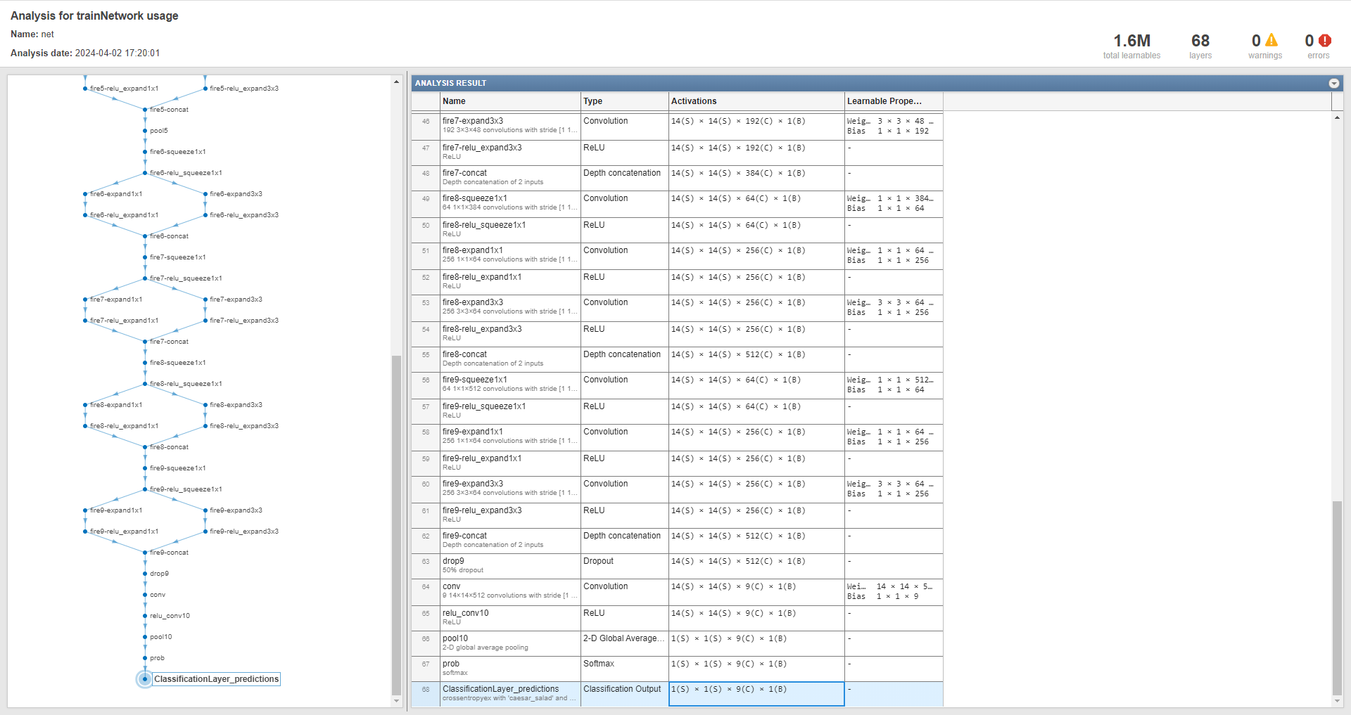
To realize image classification, this example use a SqueezeNet CNN ⁶, by built-in squeezenet function⁷, as a pre-trained network, rather than training from scratch. So, this example can be referred to as an application of Transfer Learning. We can take a look at the structure of this network using analyzeNetwork function:

1
analyzeNetwork(net)

Compare network behavior for early and later layers based on t-SNE plots

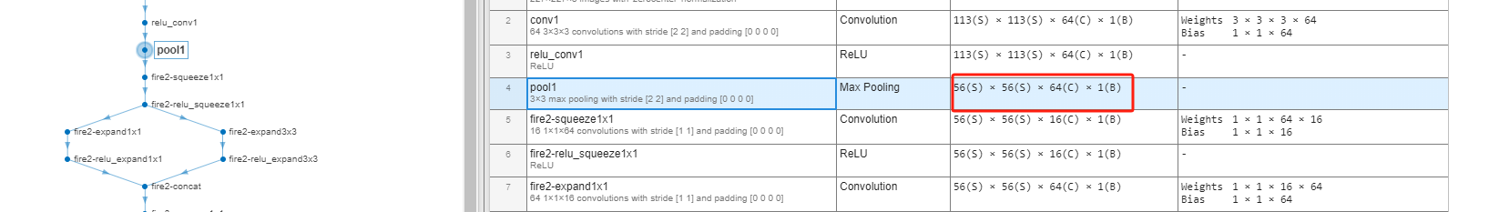
Three layers, an early max pooling layer, the final convolutional layer, and the final softmax layer, are selected for making a further analysis for network performance. Firstly, we need to activate these three layers, that is calculating the output values of the layers, using validation data set and activations function⁸.

1
2
3
4
5
6
7
8
9
10
11
12
13
clc,clear,close all
load results.mat

% Compute activations for `pool1`, `conv`, and `prob` layers
earlyLayerName = "pool1";
finalConvLayerName = "conv";
softmaxLayerName = "prob";
pool1Activations = activations(net,...
    augImdsVal,earlyLayerName,"OutputAs","rows");
finalConvActivations = activations(net,...
    augImdsVal,finalConvLayerName,"OutputAs","rows");
softmaxActivations = activations(net,...
    augImdsVal,softmaxLayerName,"OutputAs","rows");

where pool1Activations, finalConvActivations, and softmaxActivations are respectively:

1
2
3
4
5
>> whos pool1Activations finalConvActivations softmaxActivations
  Name                        Size                    Bytes  Class     Attributes
  finalConvActivations      341x1764                2406096  single              
  pool1Activations          341x200704            273760256  single              
  softmaxActivations        341x9                     12276  single   

As can be seen, for each input observation, activations function collapses all dimensions of output array of specific layer into a row vector. For example, for the above max pooling layer named pool1, the length of row vector of each observation is $200704$, which equals to $56\times56\times64\times1$:

Then, we use tsne function⁹ to reduce the dimensionality of the activation data to 2, and plot result in the two-dimensional space:

1
2
3
4
5
6
7
8
9
10
11
12
13
14
15
16
17
18
19
20
21
22
23
24
25
26
27
28
29
30
31
% Conduct t-SNE technique
rng("default") % Attention here, set the random seed for reproducibility of the t-SNE result
pool1tsne = tsne(pool1Activations);
finalConvtsne = tsne(finalConvActivations);
softmaxtsne = tsne(softmaxActivations);

% Plot t-SNE data
markerSize = 7;
classList = unique(valImds.Labels);
numClasses = length(classList);
colors = lines(numClasses);

figure("Color","w","Position",[131,342,1711,328])
tiledlayout(1,3,"TileSpacing","compact")
nexttile
hold(gca,"on"),box(gca,"on"),grid(gca,"on")
gscatter(pool1tsne(:,1),pool1tsne(:,2),valImds.Labels,colors,'.',markerSize);
title("Max pooling activations")
legend("Location","bestoutside","Interpreter","none")

nexttile
hold(gca,"on"),box(gca,"on"),grid(gca,"on")
gscatter(finalConvtsne(:,1),finalConvtsne(:,2),valImds.Labels,colors,'.',markerSize);
title("Final conv activations")
legend("Location","bestoutside","Interpreter","none")

nexttile
hold(gca,"on"),box(gca,"on"),grid(gca,"on")
gscatter(softmaxtsne(:,1),softmaxtsne(:,2),valImds.Labels,colors,'.',markerSize);
title("Softmax activations")
legend("Location","bestoutside","Interpreter","none")

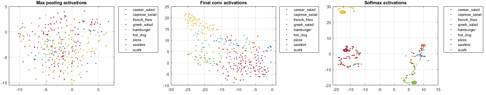
where pool1tsne, finalConvtsne, softmaxtsne are respectively:

1
2
3
4
5
>> whos pool1tsne finalConvtsne softmaxtsne
  Name                 Size            Bytes  Class     Attributes
  finalConvtsne      341x2              2728  single              
  pool1tsne          341x2              2728  single              
  softmaxtsne        341x2              2728  single           

Based on the above t-SNE plots, we can compare network behavior for early and later layers, like is described in the example documentary for example:

“The t-SNE technique (conducted by tsne function¹⁰) tries to preserve distances so that points near each other in the high-dimensional representation are also near each other in the low-dimensional representation. As shown in the confusion matrix, the network is effective at classifying into different classes. Therefore, images that are semantically similar (or of the same type), such as caesar_salad and caprese_salad, are near each other in the softmax activations space. t-SNE captures this proximity in a 2-D representation that is easier to understand and plot than the nine-dimensional softmax scores⁹, which vary from $[0,1]$.”

“Early layers tend to operate on low-level features such as edges and colors, while deeper layers have learned high-level features with more semantic meaning, such as the difference between a pizza and a hot dog. Therefore, activations from early layers do not show any clustering by class. Two images that are similar pixelwise (for example, they both contain a lot of green pixels) are near each other in the high-dimensional space of the activations, regardless of their semantic contents. Activations from later layers tend to cluster points from the same class together. This behavior is most pronounced at the softmax layer and is preserved in the two-dimensional t-SNE representation.”

“As shown in Fig. 1, the early max pooling activations do not exhibit any clustering between images of the same class. Activations of the final convolutional layer are clustered by class to some extent, but less so than the softmax activations.“

And, according to the t-SNE plot of softmax activations, we can “understand more about the structure of the posterior probability distribution. For example, the plot shows a distinct, separate cluster of French fries observations, whereas the sashimi and sushi clusters are not resolved very well. Similar to the confusion matrix, the plot suggests that the network is more accurate at predicting into the French fries class (which is consistent with the information expressed by the confusion matrix chart.)”

Analysis for observations based on t-SNE plot

A measure called ambiguity is introduced in this example. As the definition in documentation, “the ambiguity of a classification is the ratio of the second-largest probability to the largest probability. The ambiguity of a classification is between zero (nearly certain classification) and 1 (nearly as likely to be classified to the most likely class as the second class). An ambiguity of near 1 means the network is unsure of the class in which a particular image belongs. This uncertainty might be caused by two classes whose observations appear so similar to the network that it cannot learn the differences between them.”

“Or, a high ambiguity can occur because a particular observation contains elements of more than one class, so the network cannot decide which classification is correct. Note that low ambiguity does not necessarily imply correct classification; even if the network has a high probability for a class, the classification can still be incorrect.”

We can calculate ambiguities of outputs of the final softmax layer, and shows the information of 10 most ambiguous images:

1
2
3
4
5
6
7
8
9
10
11
12
13
14
15
% Calculate the ambiguity of output of the final softmax layer
[R,RI] = maxk(softmaxActivations,2,2);
ambiguity = R(:,2)./R(:,1);

% Find the most ambiguous images
[ambiguity,ambiguityIdx] = sort(ambiguity,"descend");

% View the most probable classes of the ambiguous images and the true classes
classList = unique(valImds.Labels);
top10Idx = ambiguityIdx(1:10);
top10Ambiguity = ambiguity(1:10);
mostLikely = classList(RI(ambiguityIdx,1));
secondLikely = classList(RI(ambiguityIdx,2));
table(top10Idx,top10Ambiguity,mostLikely(1:10),secondLikely(1:10),valImds.Labels(ambiguityIdx(1:10)),...
    'VariableNames',["Image #","Ambiguity","Likeliest","Second","True Class"])

The maxk function ¹¹ is to Find k largest elements of input array.

1
2
3
4
5
6
7
8
9
10
11
12
13
14
15
ans =
  10×5 table
    Image #    Ambiguity    Likeliest       Second       True Class
    _______    _________    _________    ____________    __________

       95        0.9977     sashimi      hamburger       hamburger 
      305       0.99612     sushi        pizza           sushi     
      293       0.92461     sushi        sashimi         sashimi   
      286       0.91625     sashimi      pizza           sashimi   
      127       0.90326     hamburger    french_fries    hamburger 
      186        0.8642     hamburger    pizza           pizza     
      179       0.83093     pizza        hamburger       hot_dog   
      175       0.80976     hamburger    french_fries    hot_dog   
      323        0.8015     sushi        pizza           sushi     
      178       0.79158     sashimi      hamburger       hot_dog  

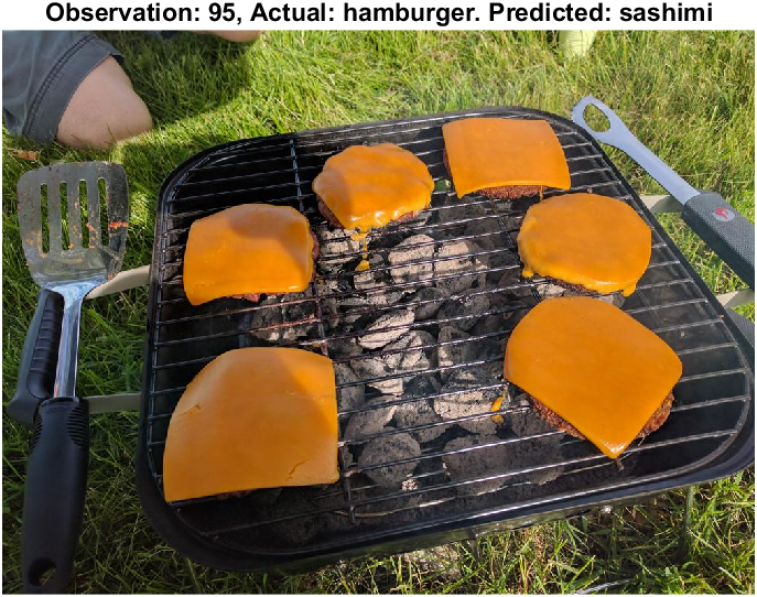
It follows that the 95th image is the most ambiguous, and it is like:

1
2
3
4
5
v = top10Idx(1);
figure("Color","w","Position",[745,410,517,424])
imshow(valImds.Files{v});
title(sprintf("Observation: %i, Actual: %s. Predicted: %s", ...
    v,string(valImds.Labels(v)),string(YPred(v))),"Interpreter","none")

We can seek out where the prediction of misclassified 95th observation locates in the t-SNE plot:

1
2
3
4
5
6
7
8
f = figure("Color","w","Position",[302,201,951,674]);
hold(gca,"on"),box(gca,"on"),grid(gca,"on")
gscatter(softmaxtsne(:,1),softmaxtsne(:,2),valImds.Labels,colors,'.',20);
title("Softmax activations")
l = legend("Location","bestoutside","Interpreter","none");

scatter(softmaxtsne(v,1),softmaxtsne(v,2), ...
    "black","LineWidth",2,"DisplayName","prediction for 95th: "+string(YPred(v)));

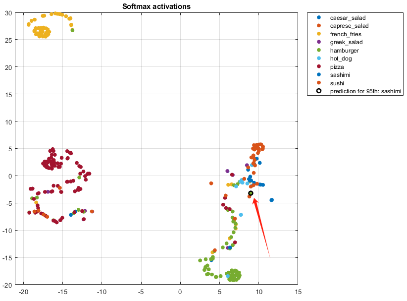
“The t-SNE plot can help to determine which images are misclassified by the network and why. And incorrect observations are often isolated points of the wrong color for their surrounding cluster.”

At last, anyway, it is a good choice to analyze the network performance by combining confusion matrix chart and t-SNE plots.

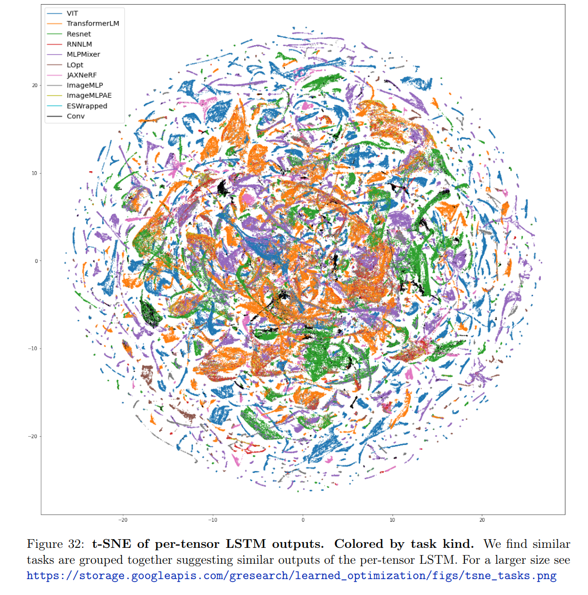
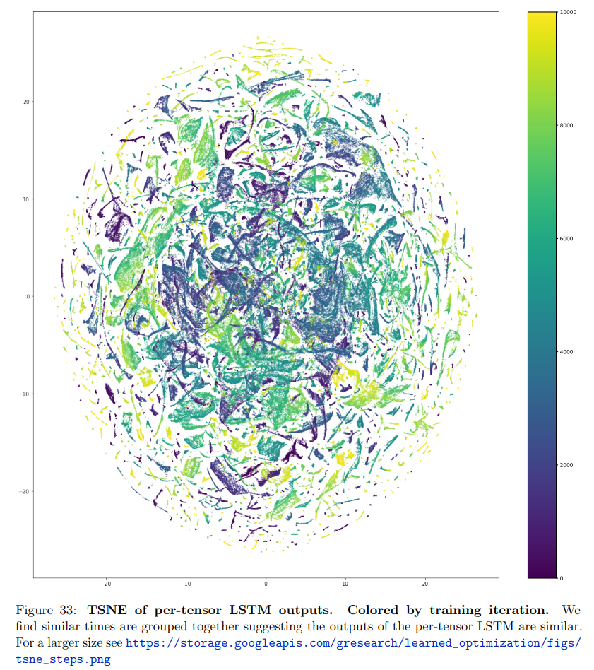
Other t-SNE applications

Two examples from Metz’s paper, Velo: Training versatile learned optimizers by scaling up¹²:

References