Central Limit Theorem (CLT)

Oct. 10, 2023

Classical CLT (Lindeberg–Lévy CLT, or Lindeberg CLT)

Let $X_1,\ X_2,\cdots,\ X_n$ denote a random sample of $n$ independent observations from a population with overall expected value $\mu$ and finite variance $\sigma^2$ ($0<\sigma^2<\infty$), then:

\[\lim_{n\rightarrow\infty}\mathrm{Pr}\Big(\dfrac1{\sqrt{n}\sigma}(\sum X_i-n\mu)\Big)=\Phi(x).\label{eq1}\]

where $\Phi(x)$ is standard normal distribution $\mathscr{N}(0,1)$, that is:

\[\Phi(x)=\dfrac1{\sqrt{2\pi}}\int_{-\infty}^{\infty}\mathrm{e}^{-t^2/2}\mathrm{d}t\notag\]

Note that:

\[\mathbb{E}(\sum X_i)=n\mu,\ \mathrm{Var}(\sum X_i)=n\sigma^2,\notag\]

so the fraction $(\sum X_i-n\mu)/(\sqrt{n}\sigma)$ in equation $\eqref{eq1}$ is the normalisation for $\sum X_i$, that is equation $\eqref{eq1}$ is equivalent to:

\[\lim_{n\rightarrow\infty}\mathrm{Pr}\Big(\sum X_i\Big)=\mathscr{N}(x\vert n\mu,n\sigma^2).\label{eq2}\]

Let $\bar{X}_n$ denote the sample mean, equation $\eqref{eq1}$ could be equivalent to:

\[\lim_{n\rightarrow\infty}\mathrm{Pr}\Big(\dfrac{\sqrt{n}}{\sigma}(\bar{X}_n-\mu)\Big)=\Phi(x).\label{eq3}\]

and equation $\eqref{eq2}$ is equivalent to:

\[\lim_{n\rightarrow\infty}\mathrm{Pr}\Big(\bar{X}_n\Big)=\mathscr{N}(x\vert \mu,\sigma^2/n). \label{eq4}\]

Equations $\eqref{eq1}$, $\eqref{eq2}$, $\eqref{eq3}$, and $\eqref{eq4}$ state that, although it is difficult to find out the specific distribution form of $X_1+X_2+\cdots+X_n$ in general cases, an approximation of which could be calculated by $\Phi(x)$ when $n$ is rather large.

For example, supposed that $\mu=1,\sigma^2=4,n=100$, we could calculate $\mathrm{Pr}(X_1+\cdots+X_{100}\le125)$ according to equation $\eqref{eq1}$, have:

\[\mathrm{Pr}(\sum_1^{100} X_i\le125)=\mathrm{Pr}\Big(\dfrac1{20}(\sum_1^{100} X_i-100)\le1.25\Big)\approx\Phi(1.25)\]

i.e.,

\[\mathrm{Pr}(\sum_1^{100} X_i\le125)\approx0.8944\]

>> normcdf(1.25,0,1)
ans =
    0.8944

MATLAB normcdf function [3].

The result $0.8944$ is of course not that accurate. Actually, there have been many existing researches about how to reduce the error, however, it needs more information about the distribution or sample moment of $X_i$.

Theorem $\eqref{eq1}$ is often called Lindeberg CLT or Lindeberg–Lévy CLT as is proved by these two scholars in 1920s. And the terminology of “Central Limit Theorem” is from this era.

De Moivre–Laplace theorem

Actually, the earliest CLT appearing in the history is a special case of theorem $\eqref{eq1}$.

Let $X_1,\ X_2,\cdots,\ X_n,\cdots$ are i.i.d., and the distribution is:

\[\mathrm{Pr}(X_i=1)=p,\ \mathrm{Pr}(X_i=0)=1-p,\]

i.e., $X_i\sim B(n,p)$ binomial distribution.

then for any real number $x$, have:

\[\lim_{n\rightarrow\infty}\mathrm{Pr}(\dfrac1{\sqrt{np(1-p)}}(X_1+\cdots+X_n-np)\le x)=\Phi(x)\label{de}\]

N.B. For binomial distribution $B(n,p)$, whose expected value is $\mathbb{E}(X_i)=p$ and variance is $\mathrm{Var}(X_i)=p(1-p)$.

Theorem $\eqref{de}$ provide a way to approximate binomial distribution by normal distribution. And it usually called De Moivre–Laplace theorem, as De Moivre discusses the case of $p=1/2$ in 1716, and Laplace promoted it to the cases of general $p$ value [2, p134].

We could simply verify this theorem as follows:

clc,clear,close all

ns = [2,5,10,1e2,1e3,1e4];
figure("Units","pixels","Position",[334,148,1290,730])
tiledlayout(2,3,"TileSpacing","compact")
for i = 1:numel(ns)
    helperPlot(ns(i),0.2)
end

function helperPlot(n,p)
x = -5:.1:5;
lefts = nan(1,numel(x));

numTimes = 1000;
for ii = 1:numel(x)
    lefts(ii) = sum((1/sqrt(n*p*(1-p)))*(binornd(n,p,1,numTimes)-n*p)<=x(ii))/numTimes;
end
rights = normcdf(x,0,1);

nexttile
hold(gca,"on"),box(gca,"on"),grid(gca,"on")
bar(x,lefts,"EdgeColor","none")
plot(x,rights,"LineWidth",1.5,"Color","k")
title(sprintf("p = %s, n = %s", num2str(p), num2str(n)))
end

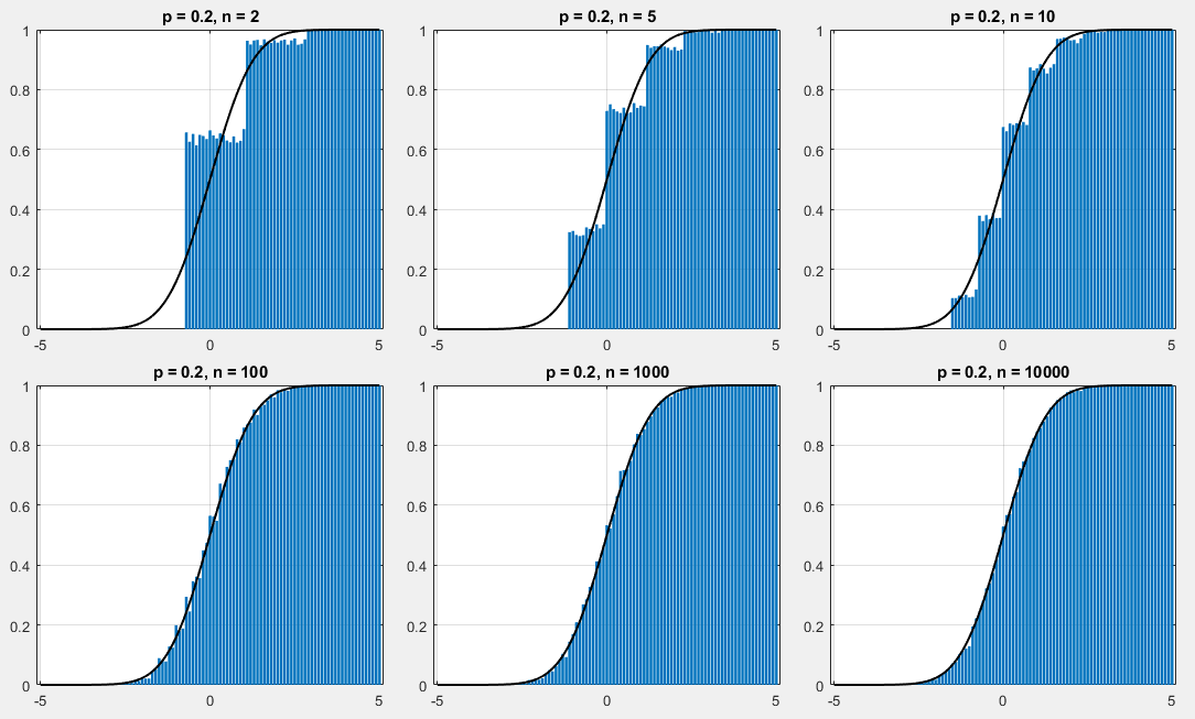
while $p=0.7$:

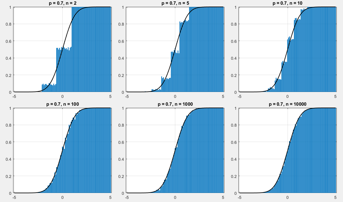
If $t_1$ and $t_2$ are two non-negative integer and $t_1<t_2$, then when $n$ is rather large, according to $\eqref{de}$, approximately have:

\[\mathrm{Pr}(t_1\le X_1+\cdots+X_n\le t_2)\approx\Phi(y_2)-\Phi(y_1)\label{eq6}\]

where

\[y_i=(t_i-np)/\sqrt{np(1-p)}\label{eq5}\]

Generally, if we correct $\eqref{eq5}$ into:

\[\begin{split} &y_1 = (t_1-\dfrac12-np)/\sqrt{np(1-p)}\\ &y_2 = (t_1+\dfrac12-np)/\sqrt{np(1-p)}\\ \end{split}\]

the accuracy of $\eqref{eq6}$ could be improved: $n$ is large, this improvement is slight, whereas $n$ is relatively small, the improvement is significant [2, p135].

Multi-dimensional CLT

The CLT could be proved using characteristic functions, and it is similar to the proof of the weak law of large numbers [4]. And the way of using characteristic function could be extended to the cases where each individual $\mathrm{\boldsymbol{X}}_i$ is a random vector in $\mathbb{R}^k$, with mean vector $\mathrm{\boldsymbol{\mu}}=\mathbb{E}(\mathrm{\boldsymbol{X}}_i)$ and covariance matrix $\boldsymbol{\Sigma}$ (among the components of the vector), and these random vectors are independent identically distributed. Summation of these vectors is being done component-wise. The multidimensional CLT states that when scaled, sums converge to a multivariate normal distribution [5, 6].

Let:

\[\mathrm{\boldsymbol{X}}_i= \begin{bmatrix} X_{i(1)}\\ \vdots\\ X_{i(k)} \end{bmatrix}\]

denote a random vector (not a random univariate variable by the way). Then the sum of the random vectors will be:

\[\sum_{i=1}^n\mathrm{\boldsymbol{X}}_i = \begin{bmatrix} X_{1(1)}\\ \vdots\\ X_{1(k)} \end{bmatrix} +\cdots+ \begin{bmatrix} X_{n(1)}\\ \vdots\\ X_{n(k)} \end{bmatrix} = \begin{bmatrix} \sum_i^nX_{i(1)}\\ \vdots\\ \sum_i^nX_{i(k)} \end{bmatrix}\]

and the average is:

\[\bar{\mathrm{\boldsymbol{X}}}_n=\dfrac1n\sum_{i=1}^n\mathrm{\boldsymbol{X}}_i\]

therefore:

\[\dfrac1{\sqrt{n}}\sum_{i=1}^n\Big(\mathrm{\boldsymbol{X}}_i-\mathbb{E}(\mathrm{\boldsymbol{X}}_i)\Big)=\dfrac1{\sqrt{n}}\Big(\mathrm{\boldsymbol{X}}_i-\boldsymbol{\mu}\Big)=\sqrt{n}\Big(\bar{\mathrm{\boldsymbol{X}}}_n-\boldsymbol{\mu}\Big)\]

The multivariate CLT states that:

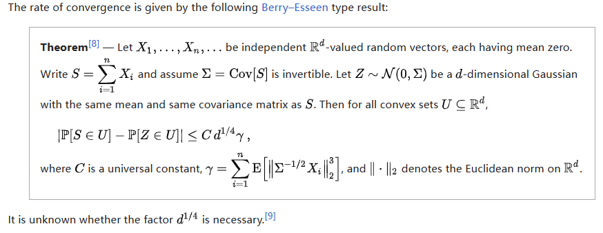
\[\sqrt{n}\Big(\bar{\mathrm{\boldsymbol{X}}}_n-\boldsymbol{\mu}\Big)\xrightarrow{\nu}\mathscr{N}_k(0,\boldsymbol{\Sigma})\]

where $\boldsymbol{\Sigma}$ is covariance matrix.

The rate of convergence is given by the following Berry-Esseen type result [4]: