MATLAB provides an easy function to add White Gaussian Noise (WGN) into original signals, i.e. awgn ¹, and whose documentation shows an example illustrating how to use it:

1
2
3
4
5
6
7
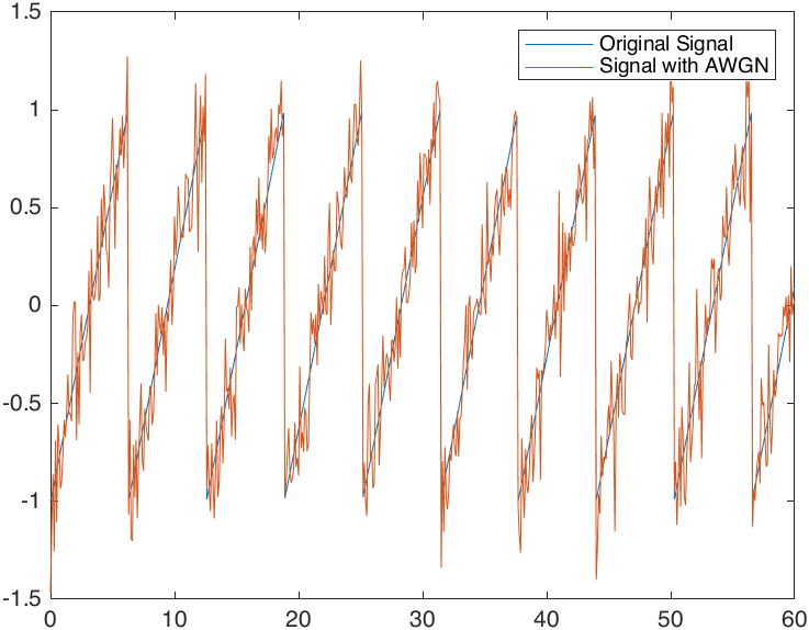
t = (0:0.1:60)';
x = sawtooth(t);

SNR_dB = 10;
y = awgn(x,SNR_dB,"measured");
plot(t,[x y])
legend("Original Signal","Signal with AWGN")

However, the documentation does not list the detailed calculation formula, and recently I plan to use this function in my research, so I want to get into it.

I debugged the awgn function step by step while running this example, and found that the main calculation codes are shown as follows:

1
2
3
4
5
6
7
8
9
10
11
12
13
function [y,noisePower] = awgn(sig,reqSNR,varargin)
% MATLAB version: 9.12.0.1884302 (R2022a)
...
sigPower = sum(abs(sig(:)).^2)/numel(sig); % linear (line 79)
...
reqSNR = 10^(reqSNR/10); % linear (line 128)
...
noisePower = sigPower/reqSNR; % linear (line 131)
...
noise = sqrt(noisePower)* randn(size(sig)); % linear (line 152)
...
y = sig + noise; % linear (line 156)
end

Supposing that $x$ and $noise$ represent input signal sig and additive white Gaussian noise, respectively, $\mathrm{SNR}_{\mathrm{dB}}$ is SNR (Signal-to-noise ratio)² in decibel unit reqSNR, we could obtain the computation expression:

i.e.,

which means that the noise is random sampled from $\mathscr{N}(0,P_{\mathrm{noise}})$, where $P_{\mathrm{noise}}$ is power of noise term. We could verify it in an easy way:

1
2
3
4
5
6
P_signal = sum(x.^2)/numel(x);
P_noise1 = P_signal/10^(SNR_dB/10); % P_signal/SNR
P_noise2 = sum((y-x).^2)/numel(x); % P_noise calculated from noise
disp(P_signal)
disp(P_noise1)
disp(P_noise1-P_noise2)

1
2
3
0.3319
0.0332
2.8030e-04

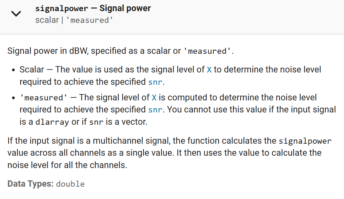
Note that in this example, the power of signal is calculated on input signal:

as the signalpower property of awgn function is set to "measured". Actually, we could specify other double value for signalpower property:

Note:

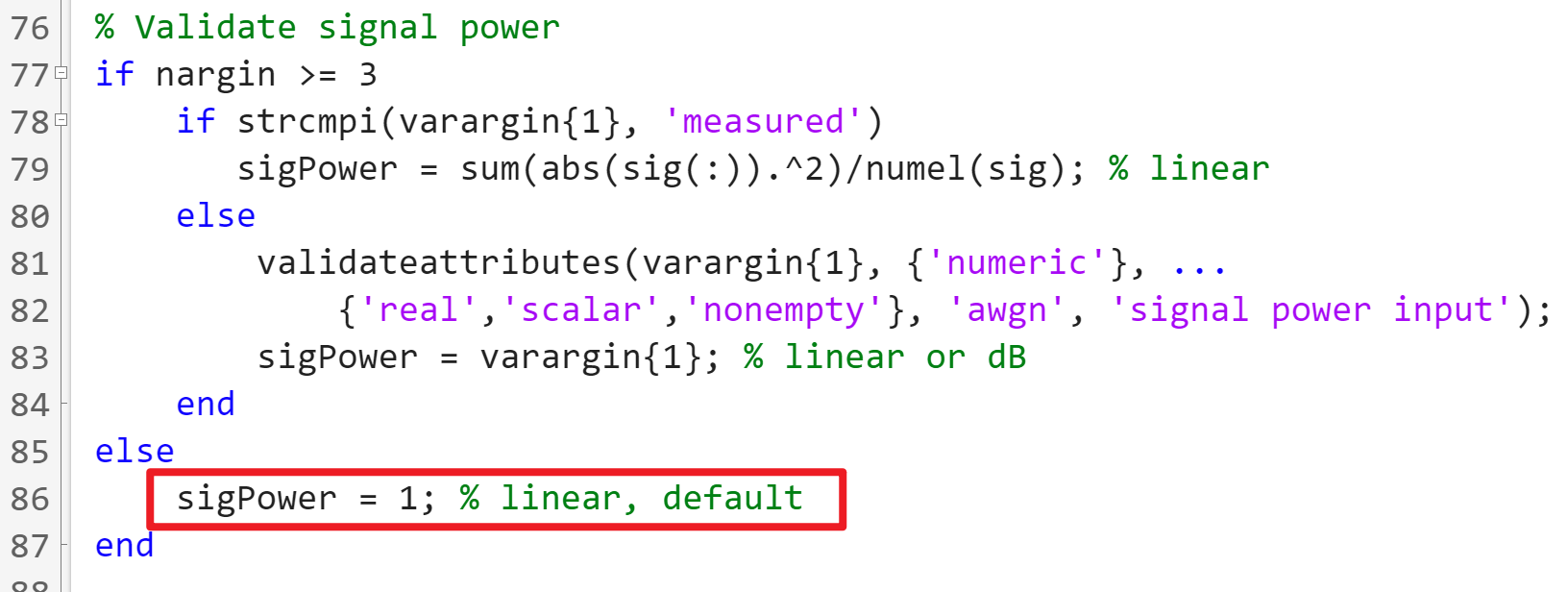
The documentation does not shows the default setting for signalpower property, but we could find that the default value is 1 from awgn source code:

For instance, signalpower could be specified as 0.8:

1
2
3
4
5
6
7
8
9
10
11
12
13
t = (0:0.1:60)';
x = sawtooth(t);

SNR_dB = 10;
sigPower = 0.8;
y = awgn(x,SNR_dB,sigPower);

P_signal = 10^(sigPower/10); % NOTE well here: unit of sigPower is dB
P_noise1 = P_signal/10^(SNR_dB/10); % P_signal/SNR
P_noise2 = sum((y-x).^2)/numel(x); % P_noise calculated from noise
disp(P_signal)
disp(P_noise1)
disp(P_noise1-P_noise2)

1
2
3
1.2023
0.1202
0.0083

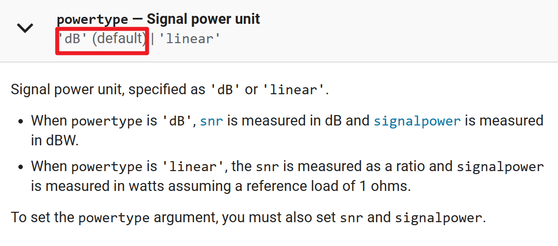
The results show that, although we set sigPower to 0.8, the value of P_signal is 1.203 instead. The reason is awgn function set default unit for sigPower to dB:

So, if want to set sigPower to 0.8 watts, we should specified as follow:

1
2
3
4
5
6
7
8
9
10
11
12
13
t = (0:0.1:60)';
x = sawtooth(t);

SNR_dB = 10;
sigPower = 0.8;
y = awgn(x,SNR_dB,sigPower,'linear');

P_signal = sigPower; % unit of sigPower is watt
P_noise1 = P_signal/10^(SNR_dB/10); % P_signal/SNR
P_noise2 = sum((y-x).^2)/numel(x); % P_noise calculated from noise
disp(P_signal)
disp(P_noise1)
disp(P_noise1-P_noise2)

1
2
3
0.8000
0.0800
6.9677e-04

References