Train Wassertein GAN with Gradient with Gradient Penalty (WGAN-GP) in MATLAB

Oct. 09, 2022

Introduction

博客¹和²介绍了MAT LAB官方提供的关于GANs的两个示例，前者介绍了无监督学习的GAN，后者介绍了有监督学习的CGAN。两个示例采用的都是来自http://download.tensorflow.org/example_images/flower_photos.tgz的鲜花数据集。本文所介绍的WGAN-GP模型(来自官方示例³)同样采用的也是该数据集，并且采用的是无监督的GAN模型。但是，本文的WGAN-GP对博客¹中的GAN做了两方面的改进：

使用Wassertein loss改进D和G的损失函数，并且使用梯度惩罚项改进D的损失函数；
更改了训练策略，使用的训练策略是训练多次D后训练一次G；

WGAN-GP的出发点源于：在理想情况下，GAN的Generator和Discriminator能够达到纳什均衡。但是，文献[2]认为，GANs中最小化的散度(i.e. negative log likelihood function)关于Generator’s learnable parameters偏导数可能是不连续的，这会导致训练困难，于是引入了Wasserstein GAN(WGAN)⁴模型，后者使用Wassertein loss来帮助稳定训练过程。但是，WGAN模型仍然会产生不良的样本或者不收敛，因为weight constraint和cost function之间的interactions会梯度停止(vanishing)和梯度爆炸(exploding)。为了解决这个问题，文献⁵引入了gradient penalty，通过惩罚具有较大norm values的梯度来改善稳定性，代价就是延长了计算时间，这个模型就是本文所述的WGAN-GP模型。

本文将重点介绍博客¹中的GAN与WGAN-GP之间的差异，相同的部分从略。

Improve Loss Function

WGAN-GP对于GAN的改进的第一个方面，就是关于损失函数。在WGAN-GP模型中，Generator和Discriminator的损失函数值计算和梯度计算是分开进行的。

For Discriminator

对于Discriminator：

function [gradientsD, lossD, lossDUnregularized] = modelGradientsD(dlnetD, dlnetG, dlX, dlZ, lambda)
% Calculate the predictions for real data with the discriminator network.
dlYPred = forward(dlnetD, dlX);

% Calculate the predictions for generated data with the discriminator
% network.
dlXGenerated = forward(dlnetG,dlZ);
dlYPredGenerated = forward(dlnetD, dlXGenerated);

% Calculate the loss.
lossDUnregularized = mean(dlYPredGenerated - dlYPred);

% Calculate and add the gradient penalty. 
epsilon = rand([1 1 1 size(dlX,4)],'like',dlX);
dlXHat = epsilon.*dlX + (1-epsilon).*dlXGenerated;
dlYHat = forward(dlnetD, dlXHat);

% Calculate gradients. To enable computing higher-order derivatives, set
% 'EnableHigherDerivatives' to true.
gradientsHat = dlgradient(sum(dlYHat),dlXHat,'EnableHigherDerivatives',true);
gradientsHatNorm = sqrt(sum(gradientsHat.^2,1:3) + 1e-10);
gradientPenalty = lambda.*mean((gradientsHatNorm - 1).^2);

% Penalize loss.
lossD = lossDUnregularized + gradientPenalty;

% Calculate the gradients of the penalized loss with respect to the
% learnable parameters.
gradientsD = dlgradient(lossD, dlnetD.Learnables);
end

正如在博客¹中所述，对于Discriminator而言，希望最大化dlYpred和-dlPredGenerated，$\tilde{Y}-Y$所对应的的损失函数mean(dlYPredGenerated-dlPred)能够做到这一点，并且避免了使用negative log likelihood function，防止了损失函数值关于Discriminator learnable parameters偏导数不连续的情况，这个损失函数就是Wasserstein损失函数。

损失函数的另一部分$\lambda(\vert\vert\nabla_{\hat{X}}\hat{Y}\vert\vert_2-1)^2$就是梯度惩罚项，就是为了防止训练时的梯度停止和梯度爆炸的情况。

以上，对于Discriminator的损失函数的改进，就是WGAN-GP模型的核心。

For Generator

对于Generator函数：

function gradientsG =  modelGradientsG(dlnetG, dlnetD, dlZ)
% Calculate the predictions for generated data with the discriminator
% network.
dlXGenerated = forward(dlnetG,dlZ);
dlYPredGenerated = forward(dlnetD, dlXGenerated);

% Calculate the loss.
lossG = -mean(dlYPredGenerated);

% Calculate the gradients of the loss with respect to the learnable
% parameters.
gradientsG = dlgradient(lossG, dlnetG.Learnables);
end

同样地，我们在博客¹中提到过，对于Generator而言，希望最大化dlYPredGenerated，损失函数-mean(dlYPredGenerated)可以做到这一点，并且避免了使用negative log likelihood function，也是WGAN的思想。

Improve Training Process

WGAN-GP对于GAN的改进的第二个方面，就是关于训练过程。博客¹中所述的GAN是每进行一次迭代(小批量数据的输入)都训练Generator和Discriminator，而本示例的WGAN-GP的训练过程则不然。

iterationG = 0;
iterationD = 0;
start = tic;

% Loop over mini-batches
while iterationG < numIterationsG
    iterationG = iterationG + 1;
    % Train discriminator only
    for n = 1:numIterationsDPerG
        iterationD = iterationD + 1;
        % Reset and shuffle mini-batch queue when there is no more data.
        if ~hasdata(mbq)
            shuffle(mbq);
        end
        % Read mini-batch of data.
        dlX = next(mbq);
        % Generate latent inputs for the generator network. Convert to
        % dlarray and specify the dimension labels 'CB' (channel, batch).
        Z = randn([numLatentInputs size(dlX,4)],'like',dlX);
        dlZ = dlarray(Z,'CB');
        % Evaluate the discriminator model gradients using dlfeval and the
        % modelGradientsD function listed at the end of the example.
        [gradientsD, lossD, lossDUnregularized] = dlfeval(@modelGradientsD, dlnetD, dlnetG, dlX, dlZ, lambda);
        % Update the discriminator network parameters.
        [dlnetD,trailingAvgD,trailingAvgSqD] = adamupdate(dlnetD, gradientsD, ...
            trailingAvgD, trailingAvgSqD, iterationD, ...
            learnRateD, gradientDecayFactor, squaredGradientDecayFactor);
    end
    % Generate latent inputs for the generator network. Convert to dlarray
    % and specify the dimension labels 'CB' (channel, batch).
    Z = randn([numLatentInputs size(dlX,4)],'like',dlX);
    dlZ = dlarray(Z,'CB');
    % Evaluate the generator model gradients using dlfeval and the
    % modelGradientsG function listed at the end of the example.
    gradientsG = dlfeval(@modelGradientsG, dlnetG, dlnetD, dlZ);
    % Update the generator network parameters.
    [dlnetG,trailingAvgG,trailingAvgSqG] = adamupdate(dlnetG, gradientsG, ...
        trailingAvgG, trailingAvgSqG, iterationG, ...
        learnRateG, gradientDecayFactor, squaredGradientDecayFactor);
...
end

从训练部分代码的主体部分可以看出，After training the discriminator for numIterationsDPerG iterations, train the generator on a single mini-batch，也就是说，Discriminator的训练次数远远多于Generator的训练次数。这种方式是认为D是更难训练的，但这不是固定的，比如博客⁶中提到说G训练多次，D训练一次。所以采用哪种训练方式还需要依据训练情况而定。

Results

使用NVIDA GeForce RTX 3060 Ti GPU 训练了2h47min，得到最终的结果：

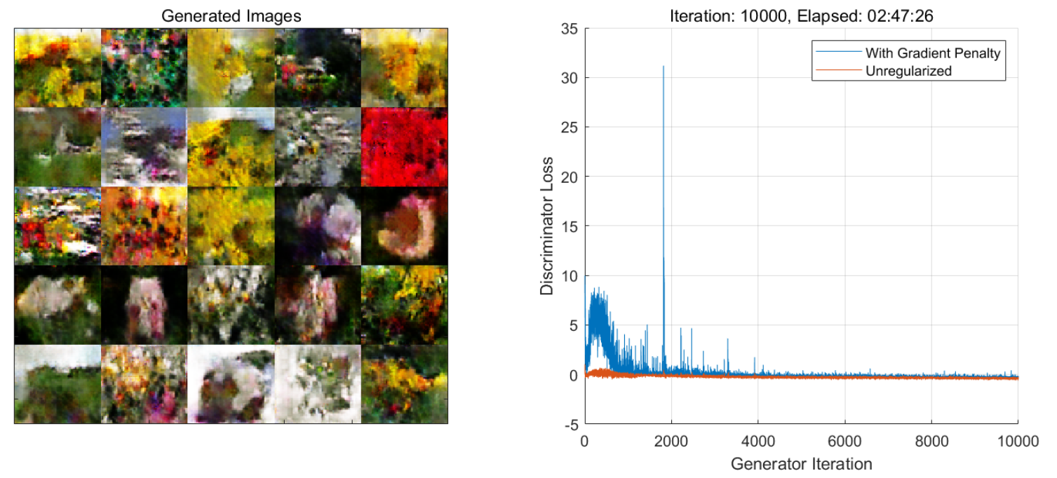
注意：这里的迭代曲线展示的是Discriminator的总的损失值lossD和不带有正则项的损失值的迭代曲线。而博客¹中的迭代曲线展示的是Generator和Discriminator的scores的迭代曲线，这一点还是有细微差别的。

查看一下生成器生成图片的效果：

% Create a dlarray object containing a batch of 25 random vectors to input to the generator network
ZNew = randn(numLatentInputs,25,'single');
dlZNew = dlarray(ZNew,'CB');

% To generate images using the GPU, also convert the data to gpuArray objects
if (executionEnvironment == "auto" && canUseGPU) || executionEnvironment == "gpu"
    dlZNew = gpuArray(dlZNew);
end

% Generate new images using the predict function with the generator and the input data
dlXGeneratedNew = predict(dlnetG,dlZNew);

% Display the images
I = imtile(extractdata(dlXGeneratedNew));
I = rescale(I);
figure
image(I)
axis off
title("Generated Images")

可以看到，本示例的WGAN-GP模型的训练时间比博客¹中GAN的训练时间1h33min长了很多，而生成图像的效果并没有改善太多。WGAN-GP作为一种GAN的改进，在一些场景下可能会好很多，但这并不是绝对的，还需要根据具体场景进行尝试。

Reference

Train Generative Adversarial Network(GAN) in MATLAB - What a starry night~. ˄ ˄² ˄³ ˄⁴ ˄⁵ ˄⁶ ˄⁷ ˄⁸
Train Conditional Generative Adversarial Network(CGAN) in MATLAB - What a starry night~. ˄
Train Wasserstein GAN with Gradient Penalty (WGAN-GP) - MathWorks. ˄
Arjovsky, Martin, Soumith Chintala, and Léon Bottou. “Wasserstein GAN.” arXiv preprint arXiv:1701.07875 (2017). ˄
Gulrajani, Ishaan, Faruk Ahmed, Martin Arjovsky, Vincent Dumoulin, and Aaron C. Courville. “Improved training of Wasserstein GANs.” In Advances in neural information processing systems, pp. 5767-5777. 2017. ˄
GAN 网络训练中，G_loss上升，D_loss下降_g loss d loss-CSDN博客. ˄