Solve Dynamical System using Neural ODE in MATLAB
Dynamical system
Introduction
在数学中,动态系统(dynamical system)1是指可以用方程来描述系统的状态变量随时间变化关系的系统。这个最普遍的定义通过允许不同的空间选择(choices of the space)和时间测量方式(how time is measured),统一了数学中的几个概念,如常微分方程(ordinary differential equations, ODEs)和遍历论(ergodic theory)。时间可以通过整数、实数、复数来测量,也可以用更普遍的代数对象(algebraic object),该代数对象不具有物理原点的记忆(losing the memory of its physical origin);空间也可以用流形(manifold)或者简单的集合,而不需要在其上定义的平滑的时空结构(smooth space-time structure)。
在给定的时间,状态空间中都有一个状态(state),该状态表征状态空间中的一个点。这个状态经常由实数元组(tuple of real numbers)或几何流形中的向量(vector in a geometrical manifold)给出。动态系统的演化规则是一个描述从当前状态到未来状态的方程。这个方程通常是确定性的(deterministic),也就是说,对于给定的时间间隔,当前状态只对应一种未来状态。然而,有一些系统是随机的(stochastic),随机时间会影响状态变量的演化。
关于“确定系统的不确定性行为”:尽管是确定性系统,在实践中,由当前状态根据演化规则推出的未来状态仍然有可能是不确定性的,因为极小的误差也会导致结果的巨大差异性。类似于解在朱利亚集上。
在物理学中,动态系统被描述为状态随时间变化的粒子(particle)或粒子系综(ensemble of particles),其状态变量服从包含时间导数的微分方程。可以通过求出微分方程的解析解,或者随时间变化的数值解来预测系统未来的行为。
动态系统的研究聚焦于动态系统理论(dynamical systems theory),该理论广泛应用于数学、物理学、生物学、化学、工程、经济学、历史和医学领域。动态系统是混沌理论(chaos theory),逻辑图动力学(logistic map dynamics)、分叉理论(bifurcation theory)、自组装和自组织过程(self-assembly and self-organization processes),以及混沌概念的边缘(the edge of chaos concept)。
Linear dynamical system
对于线性动力系统(linear dynamical systems),可以使用一些简单的方程和分类的所有轨道的行为进行求解。在线性动力系统中,相空间是一个N维欧式空间(N-dimensional Euclidean space),所有相空间内的任意一个点都可以有一个N维向量来表示。线性动力系统之所以能够很好地求解是因为它满足叠加定理(superposition principle)。
线性动力方程都可以表示为如下的形式:
\[\dot{x}=v(x)=Ax+b\label{eq1}\]其中,$x$ 为n维状态变量,$A$ 是一个矩阵,$b$ 是一个和 $x$ 相同维度的向量,$\dot{x}$ 是状态变量对时间的导数。
假设有一个简单的二自由度的线性动力系统:
\[\dot{x}=\begin{bmatrix} -0.1&-1\\ 1&-0.1\\ \end{bmatrix} x\label{eg}\]初始条件为 $x_0=[2;\ 0]$。我们可以使用 MATLAB 求解这个方程的数值解以及迭代过程,绘制出相轨迹。

1
2
3
4
5
6
7
8
9
10
11
12
13
14
15
16
17
18
19
20
21
22
23
24
25
26
27
28
29
30
31
32
33
34
clc, clear, close

x0 = [2; 0];
A = [-0.1 -1; 1 -0.1];
func = @(t, y) A*y;

numTimeSteps = 3000;
T = 50;
odeOptions = odeset(RelTol=1.e-7);
t = linspace(0, T, numTimeSteps);

[~, x]  = ode45(func, t, x0, odeOptions);

LineWidth = 1.5;
fig = figure('Position',[504, 471,1030, 420]);
subplot(1,2,1)
hold(gca, "on")
plot(t, x(:,1), LineWidth=LineWidth)
plot(t, x(:,2), LineWidth=LineWidth)
legend('$x_1(t)$', '$x_2(t)$', ...
    Interpreter='latex')
xlabel('$t$', Interpreter='latex')
ylabel('$x$', Interpreter='latex')
title('State variables varies over time')

subplot(1,2,2)
hold(gca, "on")
plot(x(:,1), x(:,2), LineWidth=LineWidth)
scatter(x0(1), x0(2), 'filled')
scatter(x(end, 1), x(end, 2), 'filled')
legend('Phase trajectory', 'Initial point', 'End point')
xlabel('$x_1$', Interpreter='latex')
ylabel('$x_2$', Interpreter='latex')
title('Phase plain')
由于式 $\eqref{eg}$ 的形式比较简单,我们可以直接求出它的解析解,看看与数值解的结果是否一致。式 $\eqref{eg}$ 可以写作:
\[\dot{x}=Ax\notag\]对上式进行拉普拉斯变换(根据微分性质),可以得到:
\[sX(s)-x(0)=AX(s)\notag\]变换可以得到:
\[X(s) = (sI-A)^{-1}x(0)\notag\]带入矩阵 $A$ 的值,可以得到:
\[\begin{align*} X(s)&=\begin{bmatrix} s+0.1&1\\ -1&s+0.1 \end{bmatrix}^{-1} \begin{bmatrix} 2\\0 \end{bmatrix}\\ &=\dfrac1{(s+0.1)^2+1} \begin{bmatrix} s+0.1&-1\\ 1&s+0.1 \end{bmatrix}\begin{bmatrix} 2\\0 \end{bmatrix}= \begin{bmatrix} \dfrac{2(s+0.1)}{(s+0.1)^2+1}\\ \dfrac2{(s+0.1)^2+1} \end{bmatrix} \end{align*}\]在对上式取拉普拉斯反变换,可以得到:
\[x(t)= \begin{bmatrix} 2e^{-0.1t}\cos(t)\\ 2e^{-0.1t}\sin(t)\\ \end{bmatrix}\label{analyticalsolution}\]式 $\eqref{analyticalsolution}$ 就是式 $\eqref{eg}$ 的解析解形式,可以根据式 $\eqref{analyticalsolution}$ 来绘制状态变量随时间变化图以及相图:

1
2
3
4
5
6
7
8
9
10
11
12
13
14
15
16
17
18
19
20
21
22
23
24
25
26
27
28
29
clc, clear, close

numpoints = 3000;
T = 50;
t = linspace(0, T, numpoints);
x1 = @(t) 2*exp(-0.1*t).*cos(t);
x2 = @(t) 2*exp(-0.1*t).*sin(t);

LineWidth = 1.5;
fig = figure('Position',[504, 471,1030, 420]);
subplot(1,2,1)
hold(gca, "on")
plot(t, x1(t), LineWidth=LineWidth)
plot(t, x2(t), LineWidth=LineWidth)
legend('$x_1(t)$', '$x_2(t)$', ...
    Interpreter='latex')
xlabel('$t$', Interpreter='latex')
ylabel('$x$', Interpreter='latex')
title('State variables varies over time')

subplot(1,2,2)
hold(gca, "on")
plot(x1(t), x2(t), LineWidth=LineWidth)
scatter(x1(t(1)), x2(t(1)), 'filled')
scatter(x1(t(end)), x2(t(end)), 'filled')
legend('Phase trajectory', 'Initial point', 'End point')
xlabel('$x_1$', Interpreter='latex')
ylabel('$x_2$', Interpreter='latex')
title('Phase plain')
可以看出,方程 $\eqref{eg}$ 的数值解形式和解析解形式的结果是一致的。
Neural ODE
Trade-off between first principle model and surrogate model (data-driven model)
在工程上,单从系统建模来说,通常有两个方向:基于第一原理建模和基于数据驱动建模。
上述准确列写出系统状态方程的过程就可以理解为第一原理建模,但有些时候,这种方式会遇到一些困难,我们会考虑使用或者部分使用数据代理模型(Surrogate model):
- 物理系统原理比较复杂或者不够清晰时,无法构建动力系统的第一原理模型
- 从实验中获得数据的难度比构建动力系统状态方程的难度小
- 第一原理模型过于复杂,求解耗时,在控制时或者是构建设备数字孪生体时有时效要求,需要加速仿真计算
- 或者单从仿真的角度讲,大规模系统的高精度批量仿真往往会消耗大量的时间
数据代理模型,也可以说是数据驱动模型,可以用神经网络模型来做。
Surrogate model for second-order linear dynamical system
仍然以式 $\eqref{eg}$ 所代表的二阶线性动力系统为例,使用 Neural ODE 为该线性动态系统建模。
Step 1: Generate real data based on state functions
1
2
3
4
5
6
7
8
9
10
x0 = [2; 0];
A = [-0.1 -1; 1 -0.1];
trueModel = @(t,y) A*y;

numTimeSteps = 2000;
T = 15;
odeOptions = odeset(RelTol=1.e-7);
t = linspace(0, T, numTimeSteps);
[~, xTrain] = ode45(trueModel, t, x0, odeOptions);
xTrain = xTrain';
Step 2: Build and initialize neural network and $\theta$ in $F(t,x(t),\theta)$
(1) Specify data length
单条数据的长度为40,但是需要41个数据点传到 dlode45 方程中,经过神经网络计算出40个点的预测值。
1
2
3
neuralOdeTimesteps = 40;
dt = t(2); % time interval
timesteps = (0:neuralOdeTimesteps)*dt; % Select the first 41 points, ie 40 time steps, of the variable 't' to pass to 'dlode45'.
(2) Initialize parameters of neural network
这里用到的神经网络有两个全连接层,其中第一个全连接层后连接一个激活函数层。

两个全连接层的权重和偏置的值都保存在结构体 neuralOdeParameters 中,并进行初始化:
1
2
3
4
5
6
7
8
9
10
11
12
13
14
neuralOdeParameters = struct;

stateSize = size(xTrain,1);
hiddenSize = 20;

neuralOdeParameters.fc1 = struct;
sz = [hiddenSize stateSize];
neuralOdeParameters.fc1.Weights = initializeGlorot(sz, hiddenSize, stateSize);
neuralOdeParameters.fc1.Bias = initializeZeros([hiddenSize 1]);

neuralOdeParameters.fc2 = struct;
sz = [stateSize hiddenSize];
neuralOdeParameters.fc2.Weights = initializeGlorot(sz, stateSize, hiddenSize);
neuralOdeParameters.fc2.Bias = initializeZeros([stateSize 1]);
上述代码在初始化权重和偏置的时候,分别使用了 initializeGlorot 和 initializeZeors 两个自定义函数:
1
2
3
4
5
6
7
8
9
10
11
12
13
14
15
16
function weights = initializeGlorot(sz,numOut,numIn,className)

arguments
    sz
    numOut
    numIn
    className = 'single'
end

Z = 2*rand(sz,className) - 1;
bound = sqrt(6 / (numIn + numOut));

weights = bound * Z;
weights = dlarray(weights);

end
其中,权重采用的是随机初始化的方式。
1
2
3
4
5
6
7
8
9
10
11
function parameter = initializeZeros(sz,className)

arguments
    sz
    className = 'single'
end

parameter = zeros(sz,className);
parameter = dlarray(parameter);

end
偏置的初始化参数则均为0。
(3) Define neural ODE model $F(t,x(t),\theta)$
1
2
3
4
5
6
7
8
9
10
function y = odeModel(~,y,theta)
% This function is passed to 'dlode45' function
% This function construct a Neural network, containing two hidden layers, ie fully-connected layer, and the first layer has a activation function
% The first hidden layer, 20-by-2,  fully-connected layer(with bias) with nonlinear activation function 'tanh'.
% The second hidden layer, 2-by-20, fully-connected layer(with bias)

y = tanh(theta.fc1.Weights*y + theta.fc1.Bias);
y = theta.fc2.Weights*y + theta.fc2.Bias;

end
(4) Define model function using dlode45
将上面所定义好的 Neural ODE 模型作为 dlode45 的输入来构建代理模型函数:
1
2
3
4
5
6
7
8
9
10
11
12
function X = model(tspan,X0,neuralOdeParameters)
% Inputs:
% tspan, 1-by-41, the first 41 time points.
% X0, 2-by-200, initial points of batches of trajectories.
% nuralOdeParameters, contains the models' weights and biases.
% Output:
% X, 2-by-200-by-40

% dlode45, built-in function, deep learning solution of nonstiff ordinary differential equation (ODE)
X = dlode45(@odeModel,tspan,X0,neuralOdeParameters,DataFormat="CB");

end
以 mini batch 中单条数据为例,分析一下这行代码所做的工作。变量 tspan 的形状是 $1\times41$,它定义41个时间点。dlode 函数通过调用用户所定义的 odeModel ,基于前一个时间点的状态变量来计算后一个时间点的状态变量,因此最终可以预测出 40 个时间节点的状态变量的值。下图展示了这一过程:

(5) Define loss function
1
2
3
4
5
6
7
8
9
10
11
12
13
14
15
16
17
18
19
20
21
22
23
24
25
function [loss,gradients] = modelLoss(tspan,X0,neuralOdeParameters,targets)
% Inputs:
% tspan, 1-by-41, the first 41 time points.
% X0, 2-by-200, initial points of batches of trajectories.
% nuralOdeParameters, contains the models' weights and biases.
% targets, 2-by-200-by-40, batches of trajectories.
% Outputs:

% Compute predictions.
% model function, custom function defined before.
% tspan, 1-by-41, the first 41 time points.
% X0, 2-by-200, initial points of batches of trajectories.
% nuralOdeParameters, contains the models' weights and biases.
% X, 2-by-200-by-40
X = model(tspan, X0, neuralOdeParameters);

% Compute L1 loss.
% X, prediction, 2-by-200-by-40
% target, real data, 2-by-200-by-40
loss = l1loss(X,targets,NormalizationFactor="all-elements",DataFormat="CBT");

% Compute gradients.
gradients = dlgradient(loss,neuralOdeParameters);

end
Step 3: Neural network training
(1) Specify parameters of Adam optimizer
1
2
3
4
5
6
7
gradDecay = 0.9;
sqGradDecay = 0.999;
learnRate = 0.002;

% Initialize the averageGrad and averageSqGrad parameters for the Adam solver.
averageGrad = [];
averageSqGrad = [];
(2) Image settings
1
2
3
4
5
6
7
8
9
10
11
12
13
14
% Every 50 iterations, solve the learned dynamics and
% display them against the ground truth in a phase diagram to show the training path.
plotFrequency = 50;

f = figure;
f.Position(3) = 2*f.Position(3);

subplot(1,2,1)
C = colororder;
lineLossTrain = animatedline(Color=C(2,:));
ylim([0 inf])
xlabel("Iteration")
ylabel("Loss")
grid on
(3) Define createMiniBatch function
1
2
3
4
5
6
7
8
9
10
11
12
13
14
15
16
17
18
19
20
21
22
23
24
function [x0, targets] = createMiniBatch(numTimesteps,numTimesPerObs,miniBatchSize,X)
% Inputs:
% numTimesteps = 2000;
% numTimesPerObs = 40;
% miniBatchSize = 200;
% X = xTrain, 2-by-2000;
% Outputs:
% x0, 2-by-200, initial points of the batches of trajectories.
% targets, 2-by-200-by-40, batches of trajectories.

% Create batches of trajectories:
% Select 200 initial points of timespan, whose length is 40(specified by 'numTimesPerObs'), in real phase trajectory,
% to construct targets.

s = randperm(numTimesteps - numTimesPerObs, miniBatchSize); % s, 1-by-200, random index in range [1, 2000-40];

x0 = dlarray(X(:, s)); % x0, 2-by-200
targets = zeros([size(X,1) miniBatchSize numTimesPerObs]); % targets, 2-by-200-by-40

for i = 1:miniBatchSize
    targets(:, i, 1:numTimesPerObs) = X(:, s(i) + 1:(s(i) + numTimesPerObs));
end

end
createMiniBatch 函数从初始值为 $[2;0]$ 的相轨迹中随机截取一些连续数据片段(数量为200个,数据片段长度为40)作为神经网络每轮训练的训练集。截取的方式是随机寻找初始点,之后选取后面的 40 个数据点作为一个片段。
注意,这个数据片段是不包括随机选取的初始点的。这么做是为了和 dlode45 的处理方式相同,这一点很重要。

另外需要注意的一行代码是:
1
2
3
...
s = randperm(numTimesteps - numTimesPerObs, miniBatchSize); % s, 1-by-200, random index in range [1, 2000-40];
...
这是随机生成初始点索引的步骤,这里删去了最后的40个数据。如果不这么做,那么后面选取数据片段的时候可能因为超出序列最大索引而报错。
(4) Model training
1
2
3
4
5
6
7
8
9
10
11
12
13
14
15
16
17
18
19
20
21
22
23
24
25
26
27
28
29
30
31
32
33
34
35
36
37
38
39
40
41
42
43
44
45
46
47
48
49
50
51
52
53
54
55
56
57
58
59
60
61
numTrainingTimesteps = numTimeSteps;
trainingTimesteps = 1:numTrainingTimesteps; % 1:2000
plottingTimesteps = 2:numTimeSteps; % 2:2000

% Train for 1200 iterations with a mini-batch-size of 200.
numIter = 1200;
miniBatchSize = 200;

start = tic;

for iter = 1:numIter

    % Create batch
    [X, targets] = createMiniBatch(numTrainingTimesteps, neuralOdeTimesteps, miniBatchSize, xTrain);
    % CreateMiniBatch: custom function
    % Inputs:
    % numTrainingTimesteps: 2000;
    % neuralOdeTimesteps: 40;
    % miniBatchsize: 200;
    % xTrain, 2-by-2000;
    % Outputs:
    % X, 2-by-200;
    % targets, 2-by-200-by-40; 200 is specified by 'miniBatchSize', 40 is spcified by 'neuralOdeTimesteps'.

    % Evaluate network and compute loss and gradients
    % Forward: calculate loss and its gradients
    [loss,gradients] = dlfeval(@modelLoss,timesteps,X,neuralOdeParameters,targets);

    % Backward: update network
    [neuralOdeParameters,averageGrad,averageSqGrad] = adamupdate(neuralOdeParameters,gradients,averageGrad,averageSqGrad,iter,...
        learnRate,gradDecay,sqGradDecay);

    % Plot loss
    subplot(1,2,1)
    currentLoss = double(loss);
    addpoints(lineLossTrain,iter,currentLoss);
    D = duration(0,0,toc(start),Format="hh:mm:ss");
    title("Elapsed: " + string(D))
    drawnow

    % Plot predicted vs. real dynamics
    if mod(iter,plotFrequency) == 0  || iter == 1
        subplot(1,2,2)

        % Use ode45 to compute the solution
        % x0=[2; 0];
        % t, the whole time span.
        y = dlode45(@odeModel,t,dlarray(x0),neuralOdeParameters,DataFormat="CB");

        % Plot real phase trajectory
        plot(xTrain(1,plottingTimesteps),xTrain(2,plottingTimesteps),"r--"), hold on
        % Plot generative phase trajectory
        plot(y(1,:),y(2,:),"b-"), hold off

        xlabel("x(1)"), ylabel("x(2)")
        title("Predicted vs. Real Dynamics")
        legend("Training Ground Truth", "Predicted")

        drawnow
    end
end
其中需要注意的一行代码是:
1
2
3
4
5
6
7
8
...
plottingTimesteps = 2:numTimeSteps; % 2:2000
...
        % Plot real phase trajectory
        plot(xTrain(1,plottingTimesteps),xTrain(2,plottingTimesteps),"r--"), hold on
        % Plot generative phase trajectory
        plot(y(1,:),y(2,:),"b-"), hold off
...
在展示真实相轨迹与模型输出相轨迹之间的对比时,作者有意没有绘制第一个点,因为在上一步骤创建 mini batch 中,无论如何选取,第一个点都不会进入训练集,因而在绘制真实数据时,也不体现初始点。
Step 4: Neural network test
在模型训练好后,需要对模型进行测试。测试的方式是将不同的初始点分别传入到 ode45 函数和训练好的 Neural ODE 中,观察两者的相轨迹是否吻合,以及它们之间的误差:
1
2
3
4
5
6
7
8
9
10
11
12
13
14
15
16
17
18
19
20
21
22
23
24
25
26
27
28
29
30
31
32
33
34
35
36
37
38
39
40
41
42
43
44
45
46
47
48
49
50
51
52
53
54
55
56
57
58
59
60
61
tPred = t;

x0Pred1 = sqrt([2;2]);
x0Pred2 = [-1;-1.5];
x0Pred3 = [0;2];
x0Pred4 = [-2;0];
x0Pred5 = [-6;0];
x0Pred6 = [-7;-7];
x0Pred7 = [5.5;6];
x0Pred8 = [9;5];

% Numerically solve the ODE true dynamics with ode45 for the four new initial conditions.
[~, xTrue1] = ode45(trueModel, tPred, x0Pred1, odeOptions);
[~, xTrue2] = ode45(trueModel, tPred, x0Pred2, odeOptions);
[~, xTrue3] = ode45(trueModel, tPred, x0Pred3, odeOptions);
[~, xTrue4] = ode45(trueModel, tPred, x0Pred4, odeOptions);
[~, xTrue5] = ode45(trueModel, tPred, x0Pred5, odeOptions);
[~, xTrue6] = ode45(trueModel, tPred, x0Pred6, odeOptions);
[~, xTrue7] = ode45(trueModel, tPred, x0Pred7, odeOptions);
[~, xTrue8] = ode45(trueModel, tPred, x0Pred8, odeOptions);

% Numerically solve the ODE with the well-trained neural ODE dynamics.
xPred1 = dlode45(@odeModel,tPred,dlarray(x0Pred1),neuralOdeParameters,DataFormat="CB");
xPred2 = dlode45(@odeModel,tPred,dlarray(x0Pred2),neuralOdeParameters,DataFormat="CB");
xPred3 = dlode45(@odeModel,tPred,dlarray(x0Pred3),neuralOdeParameters,DataFormat="CB");
xPred4 = dlode45(@odeModel,tPred,dlarray(x0Pred4),neuralOdeParameters,DataFormat="CB");
xPred5 = dlode45(@odeModel,tPred,dlarray(x0Pred5),neuralOdeParameters,DataFormat="CB");
xPred6 = dlode45(@odeModel,tPred,dlarray(x0Pred6),neuralOdeParameters,DataFormat="CB");
xPred7 = dlode45(@odeModel,tPred,dlarray(x0Pred7),neuralOdeParameters,DataFormat="CB");
xPred8 = dlode45(@odeModel,tPred,dlarray(x0Pred8),neuralOdeParameters,DataFormat="CB");

figure
subplot(4,2,1)
plotTrueAndPredictedSolutions(xTrue1, xPred1);
subplot(4,2,2)
plotTrueAndPredictedSolutions(xTrue2, xPred2);
subplot(4,2,3)
plotTrueAndPredictedSolutions(xTrue3, xPred3);
subplot(4,2,4)
plotTrueAndPredictedSolutions(xTrue4, xPred4);
subplot(4,2,5)
plotTrueAndPredictedSolutions(xTrue5, xPred5);
subplot(4,2,6)
plotTrueAndPredictedSolutions(xTrue6, xPred6);
subplot(4,2,7)
plotTrueAndPredictedSolutions(xTrue7, xPred7);
subplot(4,2,8)
plotTrueAndPredictedSolutions(xTrue8, xPred8);


function plotTrueAndPredictedSolutions(xTrue,xPred)
xPred = squeeze(xPred)';
err = mean(abs(xTrue(2:end,:) - xPred), "all");
plot(xTrue(:,1),xTrue(:,2),"r--",xPred(:,1),xPred(:,2),"b-",LineWidth=1)
title("Absolute Error = " + num2str(err,"%.4f"))
xlabel("x(1)")
ylabel("x(2)")
xlim([-2 3])
ylim([-2 3])
legend("Ground Truth","Predicted")
end
可以看到 Neural ODE 的求解效果:
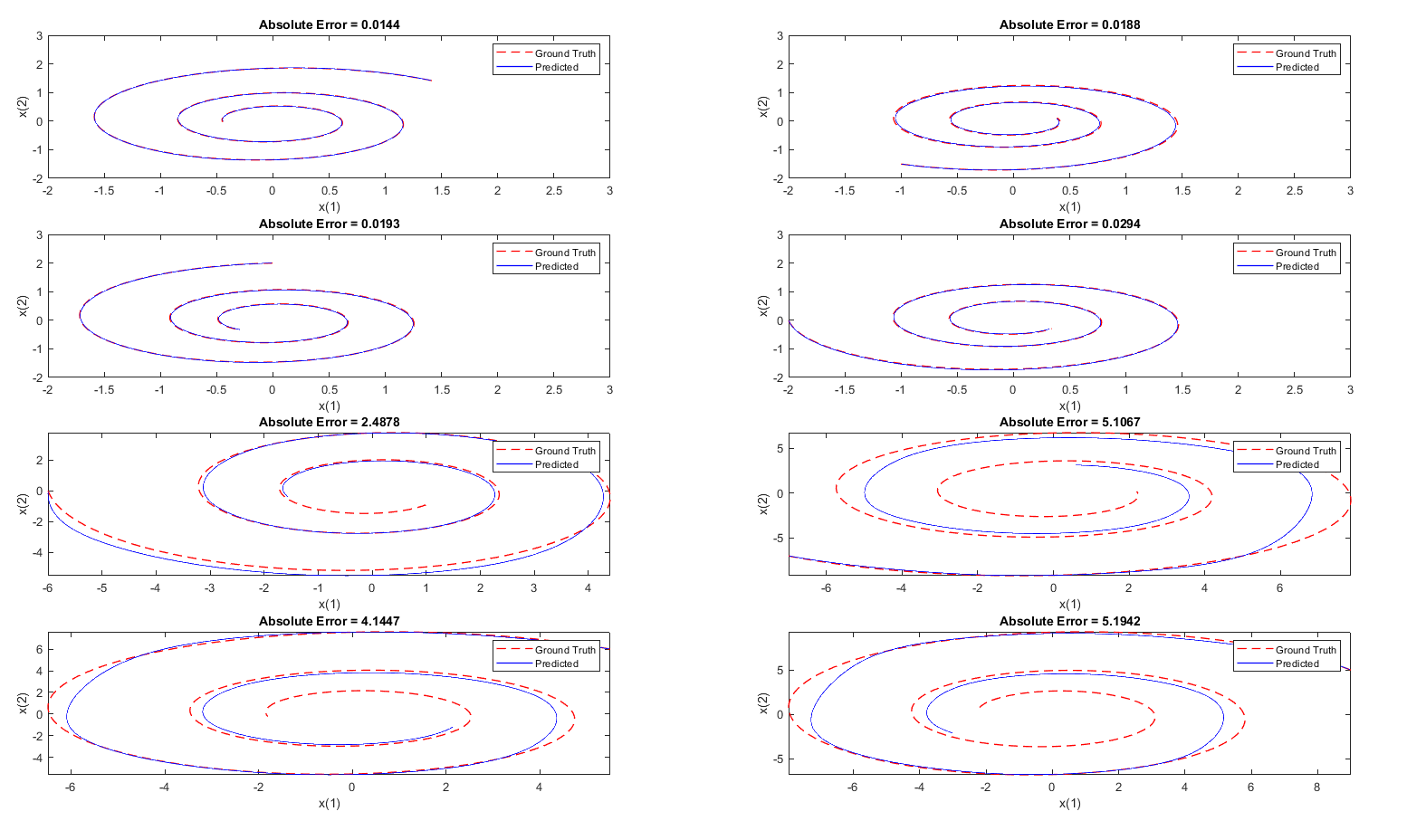
上图中的前四幅图像使用的 MATLAB 官方示例所提供的初始值,可以看到效果较好,但是后面我又随便设置了几个初始值,求解的效果并不理想。出现这种状况并不意外,这说明模型过拟合了。因为训练集的数据始终使用的是一条相轨迹,该相轨迹的初始点为 $[0,2]$ ,而我后面随便选取的分别为 $[-6;0]$,$[-7;-7]$,$[5.5;6]$,$[9;5]$ ,这和训练相轨迹的初始值差异较大,导致模型无法准确预测出相轨迹。
为了解决这个问题,可以使用以下几种方式:
- 使用多个初始值对应的相轨迹作为训练集,这体现出数据对于构建数据驱动模型的重要性
- 优化神经网络模型结构:这个例子中采用的神经网络模型是很简单的一个全连接神经网络,这样的网络并不能很好地反映时序关系,因为它的输出并不传递到输入之中。带反馈的反馈神经网络,比如 LSTM、NARX(nonlinear autoregressive network with exogenous inputs)反馈神经网络 等等是更好的选择。
虽然有一些瑕疵,但是它仍然为我们求解状态方程提供了新的思路,它有它自己的优势,这个训练好的 Neural ODE 模型可以替代 ode45 求解器对微分方程进行求解,它不需要准确的状态方程,只需要输入状态变量的初始值就可以得到一条相轨迹。
另外还有一点,上述状态方程只是一个很简单很简单的双变量线性状态方程,除此之外,还存在许多很复杂的状态方程。很多状态方程的解对于不同初始点的选取非常敏感,比如蔡氏电路2和二阶非线性电路的状态方程和相图3,Neural ODE 能否解决这样的问题?我觉得有极大的困难。使用数据驱动模型也需要对所解决的问题本身有深刻的理解,才能最大程度避免这样的风险。
In closing
总结上述过程:
- 首先需要获得真实数据,这里的真实数据是由通过数值求解状态方程得到的,除此之外还可以通过其他方式,比如开展实验、进行仿真;
- 从真实数据集中随机截取数据片段集合作为训练集;
- 在训练过程中,将 Neural ODE 的数据片段输出与训练集对应的训练数据的差异作为损失函数,并以此来降低损失函数从而达到训练 Neural ODE 模型。
References