Standard Newton’s Method, Newton’s Method with Backtracking Line-Search, vs. Gradient Descent Algorithm
Standard Newton’s method
For an unconstrained optimization:
\[\min_\boldsymbol{x} f(\boldsymbol{x})\]we can apply the second-order Taylor expansion on $f(\boldsymbol{x})$ at the $t$-th iteration (to compute $\boldsymbol{x}^{(t+1)}$):
\[\tilde{f}(\boldsymbol{x}) = f(\boldsymbol{x}^{(t)})+\nabla_\boldsymbol{x}f(\boldsymbol{x}^{(t)})(\boldsymbol{x}-\boldsymbol{x}^{(t)})+\dfrac12(\boldsymbol{x}-\boldsymbol{x}^{(t)})\nabla^2_\boldsymbol{x}f(\boldsymbol{x}^{(t)})(\boldsymbol{x}-\boldsymbol{x}^{(t)})\]To minimize $\tilde{f}(\boldsymbol{x})$, we can set its gradient as zero:
\[\nabla_\boldsymbol{x}\tilde{f}(\boldsymbol{x}) = \boldsymbol{0}\]i.e.,
\[\nabla_\boldsymbol{x}\Big(f(\boldsymbol{x}^{(t)})+\nabla_\boldsymbol{x}f(\boldsymbol{x}^{(t)})(\boldsymbol{x}-\boldsymbol{x}^{(t)})+\dfrac12(\boldsymbol{x}-\boldsymbol{x}^{(t)})\nabla^2_\boldsymbol{x}f(\boldsymbol{x}^{(t)})(\boldsymbol{x}-\boldsymbol{x}^{(t)})\Big) = \boldsymbol{0}\]then we have (note in which $\boldsymbol{x}^{(t)}$, $f(\boldsymbol{x}^{(t)})$, $\nabla_\boldsymbol{x}f(\boldsymbol{x}^{(t)})$, and $\nabla^2_\boldsymbol{x}f(\boldsymbol{x}^{(t)})$ are constants for $(t+1)$-th iteration):
\[\nabla_\boldsymbol{x}f(\boldsymbol{x}^{(t)})+\nabla^2_\boldsymbol{x}f(\boldsymbol{x}^{(t)})(\boldsymbol{x}-\boldsymbol{x}^{(t)}) = \boldsymbol{0}\]next we can derive (assuming $\nabla^2_\boldsymbol{x}f(\boldsymbol{x}^{(t)})$ is positive definite and hence full ranked):
\[\begin{split} &\nabla_\boldsymbol{x}f(\boldsymbol{x}^{(t)})+\nabla^2_\boldsymbol{x}f(\boldsymbol{x}^{(t)})(\boldsymbol{x}-\boldsymbol{x}^{(t)}) = \boldsymbol{0}\\ \Rightarrow&\nabla^2_\boldsymbol{x}f(\boldsymbol{x}^{(t)})(\boldsymbol{x}-\boldsymbol{x}^{(t)}) = -\nabla_\boldsymbol{x}f(\boldsymbol{x}^{(t)})\\ \Rightarrow&\boldsymbol{x}-\boldsymbol{x}^{(t)} = -\nabla^2_\boldsymbol{x}f(\boldsymbol{x}^{(t)})^{-1}\nabla_\boldsymbol{x}f(\boldsymbol{x}^{(t)})\\ \Rightarrow&\boldsymbol{x} = \boldsymbol{x}^{(t)}-\nabla^2_\boldsymbol{x}f(\boldsymbol{x}^{(t)})^{-1}\nabla_\boldsymbol{x}f(\boldsymbol{x}^{(t)})\\ \end{split}\]which is iterative formula, meaning that for the $(t+1)$-th iteration, we have:
\[\boldsymbol{x}^{(t+1)} = \boldsymbol{x}^{(t)}-\nabla^2_\boldsymbol{x}f(\boldsymbol{x}^{(t)})^{-1}\nabla_\boldsymbol{x}f(\boldsymbol{x}^{(t)})\label{eq1}\]This, iteration formula $\eqref{eq1}$, is actually the standard Newton algorithm for unconstrained minimization1.
Btw, the form $\eqref{eq1}$ looks like the way when using Multi-variate Newton method to solve non-linear systems of equations2, but they are slightly different; during derivation, the former is to set the gradient of the Taylor expansion is 0, and the latter is to set the Taylor expansion per se as 0.
Newton’s method with backtracking line-search
If the given initial point is near the minimum, Newton’s method converges quickly, but when the initial point is improper, far from the minimum, Newton’s method may diverge.
The line-search procedure is a remedy to solve this problem. Define the search direction as $\boldsymbol{d}$:
\[\boldsymbol{d}:=-\nabla^2_\boldsymbol{x}f(\boldsymbol{x}^{(t)})^{-1}\nabla_\boldsymbol{x}f(\boldsymbol{x}^{(t)})\label{eq3}\]then the Newton’s method $\eqref{eq1}$ can be written as:
\[\boldsymbol{x}^{(t+1)} = \boldsymbol{x}^{(t)}+\boldsymbol{d}\]At this time, we can add a line-search procedure, which is an algorithm for finding an appropriate step size $\gamma\ge0$ to make iteration formula:
\[\boldsymbol{x}^{(t+1)} = \boldsymbol{x}^{(t)}+\gamma\cdot\boldsymbol{d}\]ensure function $f$ decreases by a sufficient amount during each iteration.
There are many methods to design such a line-search procedure, and one is called backtracking line search. First, we initially set $\gamma$ to 1 and iteratively reduces $\gamma$ by a factor $\beta$ until $f(\boldsymbol{x}^{(t)}+\gamma\cdot\boldsymbol{d})$ is sufficiently smaller than $f(\boldsymbol{x}^{(t)})$, i.e., $f(\boldsymbol{x}^{(t)}+\gamma\cdot\boldsymbol{d})-f(\boldsymbol{x}^{(t)})$ less than a certain value. One way is to make:
\[f(\boldsymbol{x}^{(t)}+\gamma\cdot d)-f(\boldsymbol{x}^{(t)})\le\gamma\cdot\alpha\cdot\nabla_\boldsymbol{x}f(\boldsymbol{x}^{(t)})^T\boldsymbol{d}\]i.e.,
\[f(\boldsymbol{x}^{(t)}+\gamma\cdot d)\le f(\boldsymbol{x}^{(t)})+\gamma\cdot\alpha\cdot\nabla_\boldsymbol{x}f(\boldsymbol{x}^{(t)})^T\boldsymbol{d}\label{eq2}\]where $\alpha$ is a constant. Relationship $\eqref{eq2}$ is also called as Armijo–Goldstein condition 3 (or Armijo-Goldstein inequality4).
The shrinking continues until a value is found that is small enough to provide a decrease in the objective function that adequately matches the decrease that is expected to be achieved, based on the local function gradient $\nabla_\boldsymbol{x}f(\boldsymbol{x}^{(t)})$.3
If the inequality doesn’t hold, then we shrink the $\gamma$ by a factor $\beta$:
\[\gamma\leftarrow\beta\cdot\gamma\label{eq4}\]In $\eqref{eq2}$, for $f(\boldsymbol{x}^{(t)})^T\boldsymbol{d}$, we have:
\[\nabla_\boldsymbol{x}f(\boldsymbol{x}^{(t)})^T\boldsymbol{d} = -\nabla_\boldsymbol{x}f(\boldsymbol{x}^{(t)})^T\nabla^2_\boldsymbol{x}f(\boldsymbol{x}^{(t)})^{-1}\nabla_\boldsymbol{x}f(\boldsymbol{x}^{(t)})\]because $\nabla^2_\boldsymbol{x}f(\boldsymbol{x}^{(t)})$ is assumed as positive definite before, $f(\boldsymbol{x}^{(t)})^T\boldsymbol{d}$ is always negative. Hence, intuitively, the relationship $\eqref{eq2}$ states that $f(\boldsymbol{x}^{(t)}+\gamma\cdot d)-f(\boldsymbol{x}^{(t)})$ must be less than or equal to a negative number, meaning the most updated $f(\boldsymbol{x}^{(t)}+\gamma\cdot\boldsymbol{d})$ must be less than $f(\boldsymbol{x}^{(t)})$, otherwise we need to shrink step size till the $\eqref{eq2}$ is satisfied. So, this method can effectively prevent Newton’s method diverging.
Btw, I mainly refer1 when writing this blog, and whose derivation for backtracking line search shows as follows:
As can be seen, here the search direction is defined as:
\[\boldsymbol{d}:=\nabla^2_\boldsymbol{x}f(\boldsymbol{x}^{(t)})^{-1}\nabla_\boldsymbol{x}f(\boldsymbol{x}^{(t)})\]i.e., not including a negative sign. But in his pseudocode block, on the right side of the inequality, it seems that there should be a minus sign before $\gamma\cdot\alpha\cdot\nabla_\boldsymbol{x}f(\boldsymbol{x}^{(t)})^T\boldsymbol{d}$ instead of a plus sign, i.e., the right side should be:
\[f(\boldsymbol{x}^{(t)})-\gamma\cdot\alpha\cdot\nabla_\boldsymbol{x}f(\boldsymbol{x}^{(t)})^T\boldsymbol{d}\]So, I think this is a small mistake. And it is more common to define the line-search direction as a decreasing direction, i.e., $\eqref{eq3}$.34
Gradient descent algorithm
The standard Newton algorithm $\eqref{eq1}$ is different from gradient descent (GD) algorithm5:
\[\boldsymbol{x}^{(t+1)} = \boldsymbol{x}^{(t)}-\gamma \nabla_\boldsymbol{x}f(\boldsymbol{x}^{(t)})\]where $\gamma$ is the step size. The idea of GD is “the gradient always points in the upward direction of the function”. And we can feel that Newton algorithm $\eqref{eq1}$ is with more computation complexity, because it needs to compute Hessian matrix6.
Case study
Next, by taking two examples, we’ll use above three algorithms to find the minimum.
Example 1: Quadratic equation
Consider such a quadratic equation:
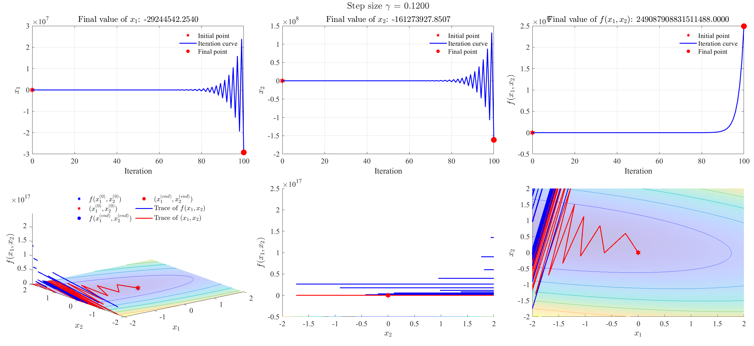
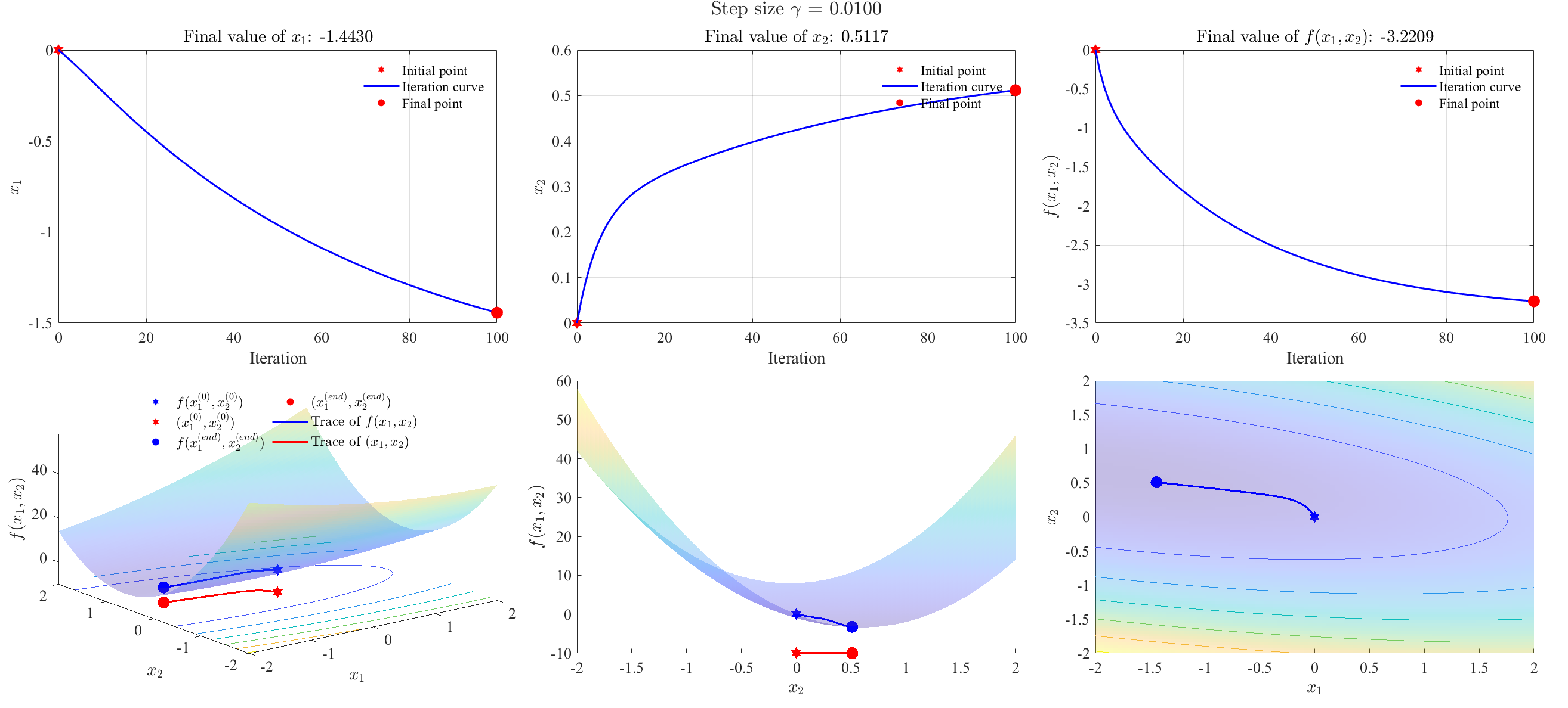
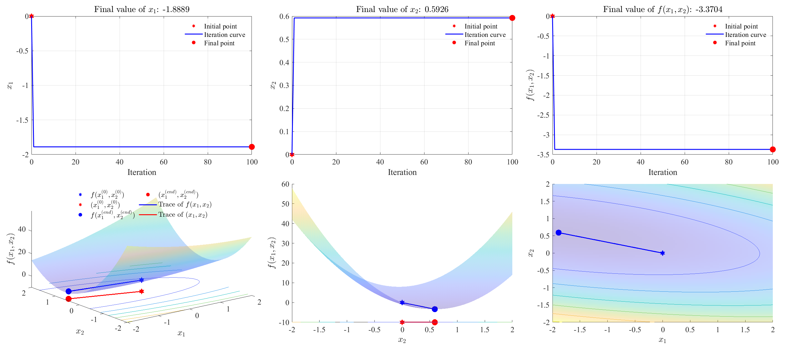
\[f(x_1, x_2) = x_1^2+3x_1x_2+9x_2^2+2x_1-5x_2\]Select $\boldsymbol{x}^{(0)} = [0,0]^T$, and maximum iteration is 100.
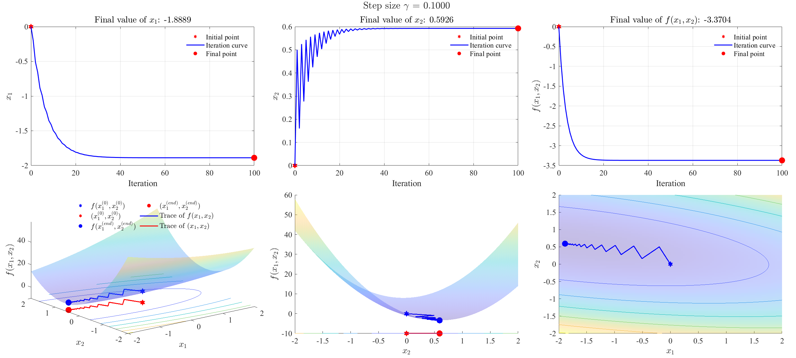
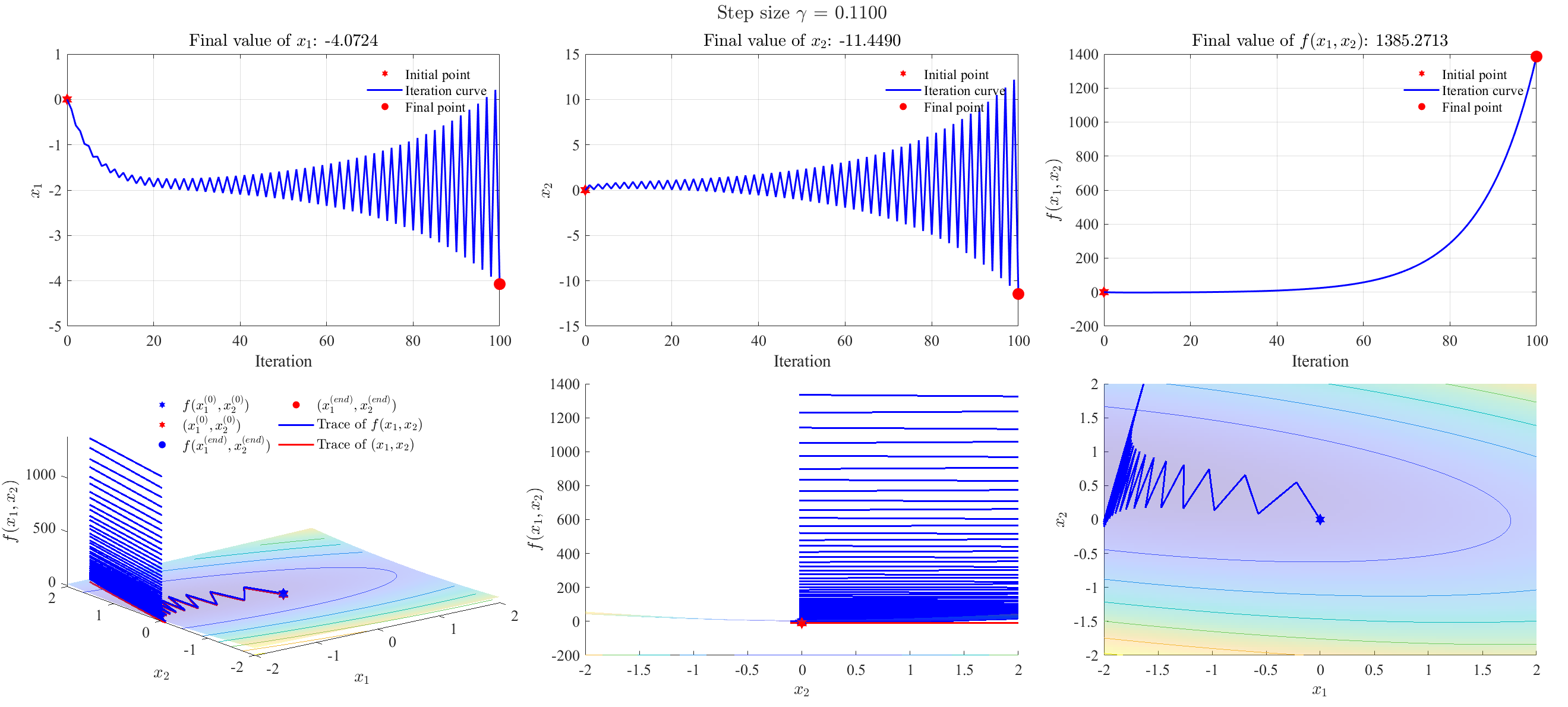
Gradient descent algorithm
Step size = 0.1 (properly convergent)
1
2
3
4
5
6
7
8
9
10
11
12
13
14
15
16
17
18
19
20
21
22
23
24
25
26
27
28
29
30
31
32
33
34
35
36
37
38
39
40
41
42
43
44
45
46
47
48
49
50
51
52
53
54
55
56
57
58
59
60
61
62
63
64
65
66
67
68
69
70
71
72
73
74
75
76
77
78
79
80
81
82
83
84
85
86
87
88
89
90
91
92
93
94
95
96
97
98
99
100
101
102
103
104
105
106
107
108
109
110
111
112
113
114
115
116
117
118
119
120
121
122
123
124
125
126
127
128
129
130
131
132
133
134
135
136
137
138
139
140
141
142
143
144
145
146
147
148
149
150
151
152
153
154
155
156
157
158
159
160
161
162
163
164
165
166
167
168
169
170
171
172
173
174
175
176
177
clc, clear, close all

syms x1 x2
f_sym = x1.^2+3*x1.*x2+9*x2.^2+2*x1-5*x2;

g_sym = gradient(f_sym, [x1, x2]);

f = matlabFunction(f_sym, 'Vars', {x1, x2});
g = matlabFunction(g_sym, 'Vars', {x1, x2});

x0 = [0, 0]';
stepSz = 0.1;
helperGD(f, g, stepSz, x0)

function helperGD(f, g, gamma, x0)
xOld = x0;
numIter = 100;

xk = nan(numIter, 2);
iters = (1:numIter)';

for i = 1:numIter
    % ============ Gradient descent ============
    gi = g(xOld(1), xOld(2));
    xNew = xOld-gamma*gi;
    % ====================================

    xk(i,:) = xNew;
    xOld = xNew;

    % % Stop if diverge
    % if f(xNew(1), xNew(2))>1e5
    %     break
    % end

    % % Early stop if converge
    % if i>1 && norm(f(xk(i,1), xk(i,2)) - f(xk(i-1,1), xk(i-1,2)))<=1e-4
    %     xk(i+1:end, :) = [];
    %     iters(i+1:end) = [];
    %     break
    % end
end

xk(isnan(xk)) = [];

xs1 = [x0(1); xk(:,1)];
xs2 = [x0(2); xk(:,2)];
iters = [0; iters(1:(height(xs1)-1))];
fs = f(xs1, xs2);

fprintf('Final function value: %.4f\n', f(xNew(1), xNew(2)))

% Present results
helperPlot(f, gamma, xs1, xs2, iters, fs)
end

function helperPlot(f, gamma, xs1, xs2, iters, fs)
figure('Color', 'w', 'Position', [305,283,1915,835])
tiledlayout(2, 3, 'TileSpacing', 'compact')
LineWidth = 1.5;
FontSize = 13;
FontName = 'Times New Roman';

%% Axes 1
nexttile
hold(gca, 'on'), grid(gca, 'on'), box(gca, 'on')
scatter(iters(1), xs1(1), 100, 'Marker', 'hexagram', ...
    'MarkerFaceColor', 'r', 'MarkerEdgeColor', 'none', 'DisplayName', 'Initial point')
plot(iters, xs1, 'LineWidth', LineWidth, 'Color', 'b', 'DisplayName', 'Iteration curve')
scatter(iters(end), xs1(end), 100, 'Marker', 'o', ...
    'MarkerFaceColor', 'r', 'MarkerEdgeColor', 'none', 'DisplayName', 'Final point')
xlabel('Iteration')
ylabel('$x_1$', 'Interpreter', 'latex')
legend('Box', 'off')
title(sprintf('Final value of %s: %.4f', '$x_1$', xs1(end)), 'Interpreter', 'latex')
set(gca, 'FontSize', FontSize, 'FontName', FontName)

%% Axes 2
nexttile
hold(gca, 'on'), grid(gca, 'on'), box(gca, 'on')
scatter(iters(1), xs2(1), 100, 'Marker', 'hexagram', ...
    'MarkerFaceColor', 'r', 'MarkerEdgeColor', 'none', 'DisplayName', 'Initial point')
plot(iters, xs2, 'LineWidth', LineWidth, 'Color', 'b', 'DisplayName', 'Iteration curve')
scatter(iters(end), xs2(end), 100, 'Marker', 'o', ...
    'MarkerFaceColor', 'r', 'MarkerEdgeColor', 'none', 'DisplayName', 'Final point')
xlabel('Iteration')
ylabel('$x_2$', 'Interpreter', 'latex')
legend('Box', 'off')
title(sprintf('Final value of %s: %.4f', '$x_2$', xs2(end)), 'Interpreter', 'latex')
set(gca, 'FontSize', FontSize, 'FontName', FontName)

%% Axes 3
nexttile
hold(gca, 'on'), grid(gca, 'on'), box(gca, 'on')
scatter(iters(1), fs(1), 100, 'Marker', 'hexagram', ...
    'MarkerFaceColor', 'r', 'MarkerEdgeColor', 'none', 'DisplayName', 'Initial point')
plot(iters, fs, 'LineWidth', LineWidth, 'Color', 'b', 'DisplayName', 'Iteration curve')
scatter(iters(end), fs(end), 100, 'Marker', 'o', ...
    'MarkerFaceColor', 'r', 'MarkerEdgeColor', 'none', 'DisplayName', 'Final point')
xlabel('Iteration')
ylabel('$f(x_1,x_2)$', 'Interpreter', 'latex')
legend('Box', 'off')
title(sprintf('Final value of %s: %.4f', '$f(x_1,x_2)$', fs(end)), 'Interpreter', 'latex')
set(gca, 'FontSize', FontSize, 'FontName', FontName)

%% Axes 4
nexttile
view(3)
hold(gca, 'on')
ax1 = gca();

x_min = -2;
x_max = 2;
x1 = linspace(x_min, x_max, 100);
x2 = linspace(x_min, x_max, 100);

[X1, X2] = meshgrid(x1, x2);
y = f(X1, X2);
sc = surfc(X1, X2, y, 'FaceAlpha', 0.3, 'EdgeColor', 'none', 'DisplayName', '$f(x_1,x_2)$', 'HandleVisibility', 'off');
sc(2).HandleVisibility = 'off';
sc(2).LevelList = min(y,[],"all"):10:max(y,[],"all");
LevelStep = sc(2).LevelStep;

scatter3(xs1(1), xs2(1), fs(1), 100, 'Marker', 'hexagram', ...
    'MarkerFaceColor', 'b', 'MarkerEdgeColor', 'none', 'DisplayName', '$f(x_1^{(0)}, x_2^{(0)})$')
scatter3(xs1(1), xs2(1), -LevelStep, 100, 'Marker', 'hexagram', ...
    'MarkerFaceColor', 'r', 'MarkerEdgeColor', 'none', 'DisplayName', '$(x_1^{(0)}, x_2^{(0)})$')
scatter3(xs1(end), xs2(end), fs(end), 100, 'Marker', 'o', ...
    'MarkerFaceColor', 'b', 'MarkerEdgeColor', 'none', 'DisplayName', '$f(x_1^{(end)}, x_2^{(end)})$')
scatter3(xs1(end), xs2(end), -LevelStep, 100, 'Marker', 'o', ...
    'MarkerFaceColor', 'r', 'MarkerEdgeColor', 'none', 'DisplayName', '$(x_1^{(end)}, x_2^{(end)})$')

plot3(xs1, xs2, fs, 'LineWidth', LineWidth, 'Color', 'b', 'DisplayName', 'Trace of $f(x_1,x_2)$')
plot3(xs1, xs2, -LevelStep*ones(size(xs1)), 'LineWidth', LineWidth, 'Color', 'r', 'DisplayName', 'Trace of $(x_1,x_2)$')
% helperFill3(xs1, xs2, fs, xs1, xs2, -LevelStep*ones(size(xs1)), 'g')

xlim([x_min, x_max])
ylim([x_min, x_max])
xlabel('$x_1$', 'Interpreter', 'latex')
ylabel('$x_2$', 'Interpreter', 'latex')
zlabel('$f(x_1,x_2)$', 'Interpreter', 'latex')
lgd1 = legend('Interpreter', 'latex', 'Box', 'off', 'NumColumns', 2, 'Location', 'north', 'EdgeColor', 'none');
set(gca, 'FontSize', FontSize, 'FontName', FontName)

%% Axes 5
nexttile
ax2 = gca();
copyobj(allchild(ax1), ax2);
view([90,0])
xlim([x_min, x_max])
ylim([x_min, x_max])
xlabel('$x_1$', 'Interpreter', 'latex')
ylabel('$x_2$', 'Interpreter', 'latex')
zlabel('$f(x_1,x_2)$', 'Interpreter', 'latex')
% legend(ax2, lgd1.String, 'Interpreter', lgd1.Interpreter, ...
%     'Box', lgd1.Box, 'NumColumns', lgd1.NumColumns, ...
%     'Location', lgd1.Location, 'EdgeColor', lgd1.EdgeColor);
set(ax2, 'FontSize', FontSize, 'FontName', FontName)

%% Axes 6
nexttile
ax3 = gca();
copyobj(allchild(ax1), ax3);
view([0,90])
xlim([x_min, x_max])
ylim([x_min, x_max])
xlabel('$x_1$', 'Interpreter', 'latex')
ylabel('$x_2$', 'Interpreter', 'latex')
zlabel('$f(x_1,x_2)$', 'Interpreter', 'latex')
% legend(ax3, lgd1.String, 'Interpreter', lgd1.Interpreter, ...
%     'Box', lgd1.Box, 'NumColumns', lgd1.NumColumns, ...
%     'Location', lgd1.Location, 'EdgeColor', lgd1.EdgeColor);
set(gca, 'FontSize', FontSize, 'FontName', FontName)

sgtitle(sprintf('Step size %s = %.4f', "$\gamma$", gamma), 'Interpreter', 'latex', ...
    'FontSize', FontSize+3, 'FontName', FontName)
end
Step size = 0.11 (divergent)
Step size = 0.12 (divergent)
Step size = 0.01 (slowly convergent)
Newton’s method
1
2
3
4
5
6
7
8
9
10
11
12
13
14
15
16
17
18
19
20
21
22
23
24
25
26
27
28
29
30
31
32
33
34
35
36
37
38
39
40
41
42
43
44
45
46
47
48
49
50
51
52
53
54
55
56
57
58
59
60
61
62
63
64
65
66
67
68
69
70
71
72
73
74
75
76
77
78
79
80
81
82
83
84
85
86
87
88
89
90
91
92
93
94
95
96
97
98
99
100
101
102
103
104
105
106
107
108
109
110
111
112
113
114
115
116
117
118
119
120
121
122
123
124
125
126
127
128
129
130
131
132
133
134
135
136
137
138
139
140
141
142
143
144
145
146
147
148
149
150
151
152
153
154
155
156
157
158
159
160
161
162
163
164
165
166
167
168
169
170
171
172
173
174
175
176
177
clc, clear, close all

syms x1 x2
f_sym = x1.^2+3*x1.*x2+9*x2.^2+2*x1-5*x2;

g_sym = gradient(f_sym, [x1, x2]);
H_sym = hessian(f_sym, [x1, x2]);

f = matlabFunction(f_sym, 'Vars', {x1, x2});
g = matlabFunction(g_sym, 'Vars', {x1, x2});
H = matlabFunction(H_sym, 'Vars', {x1, x2});

x0 = [0, 0]';
helperNewton(f, g, H, x0)

function helperNewton(f, g, H, x0)
xOld = x0;
numIter = 100;

xk = nan(numIter, 2);
iters = (1:numIter)';

for i = 1:numIter
    %  ============ Newton's method ============
    gi = g(xOld(1), xOld(2));
    Hi = H(xOld(1), xOld(2));

    xNew = xOld-Hi\gi;
    % =====================================

    xk(i,:) = xNew;
    xOld = xNew;

    % % Stop if diverge
    % if f(xNew(1), xNew(2))>100
    %     break
    % end
    %
    % % Early stop if converge
    % if i>1 && norm(f(xk(i,1), xk(i,2)) - f(xk(i-1,1), xk(i-1,2)))<=1e-4
    %     xk(i+1:end, :) = [];
    %     iters(i+1:end) = [];
    %     break
    % end
end

xk(isnan(xk)) = [];

xs1 = [x0(1); xk(:,1)];
xs2 = [x0(2); xk(:,2)];
iters = [0; iters(1:(height(xs1)-1))];
fs = f(xs1, xs2);

fprintf('Final function value: %.4f\n', f(xNew(1), xNew(2)))

% Present results
helperPlot(f, xs1, xs2, iters, fs)
end

function helperPlot(f, xs1, xs2, iters, fs)
figure('Color', 'w', 'Position', [305,283,1915,835])
tiledlayout(2, 3, 'TileSpacing', 'compact')
LineWidth = 1.5;
FontSize = 13;
FontName = 'Times New Roman';

%% Axes 1
nexttile
hold(gca, 'on'), grid(gca, 'on'), box(gca, 'on')
scatter(iters(1), xs1(1), 100, 'Marker', 'hexagram', ...
    'MarkerFaceColor', 'r', 'MarkerEdgeColor', 'none', 'DisplayName', 'Initial point')
plot(iters, xs1, 'LineWidth', LineWidth, 'Color', 'b', 'DisplayName', 'Iteration curve')
scatter(iters(end), xs1(end), 100, 'Marker', 'o', ...
    'MarkerFaceColor', 'r', 'MarkerEdgeColor', 'none', 'DisplayName', 'Final point')
xlabel('Iteration')
ylabel('$x_1$', 'Interpreter', 'latex')
legend('Box', 'off')
title(sprintf('Final value of %s: %.4f', '$x_1$', xs1(end)), 'Interpreter', 'latex')
set(gca, 'FontSize', FontSize, 'FontName', FontName)

%% Axes 2
nexttile
hold(gca, 'on'), grid(gca, 'on'), box(gca, 'on')
scatter(iters(1), xs2(1), 100, 'Marker', 'hexagram', ...
    'MarkerFaceColor', 'r', 'MarkerEdgeColor', 'none', 'DisplayName', 'Initial point')
plot(iters, xs2, 'LineWidth', LineWidth, 'Color', 'b', 'DisplayName', 'Iteration curve')
scatter(iters(end), xs2(end), 100, 'Marker', 'o', ...
    'MarkerFaceColor', 'r', 'MarkerEdgeColor', 'none', 'DisplayName', 'Final point')
xlabel('Iteration')
ylabel('$x_2$', 'Interpreter', 'latex')
legend('Box', 'off')
title(sprintf('Final value of %s: %.4f', '$x_2$', xs2(end)), 'Interpreter', 'latex')
set(gca, 'FontSize', FontSize, 'FontName', FontName)

%% Axes 3
nexttile
hold(gca, 'on'), grid(gca, 'on'), box(gca, 'on')
scatter(iters(1), fs(1), 100, 'Marker', 'hexagram', ...
    'MarkerFaceColor', 'r', 'MarkerEdgeColor', 'none', 'DisplayName', 'Initial point')
plot(iters, fs, 'LineWidth', LineWidth, 'Color', 'b', 'DisplayName', 'Iteration curve')
scatter(iters(end), fs(end), 100, 'Marker', 'o', ...
    'MarkerFaceColor', 'r', 'MarkerEdgeColor', 'none', 'DisplayName', 'Final point')
xlabel('Iteration')
ylabel('$f(x_1,x_2)$', 'Interpreter', 'latex')
legend('Box', 'off')
title(sprintf('Final value of %s: %.4f', '$f(x_1,x_2)$', fs(end)), 'Interpreter', 'latex')
set(gca, 'FontSize', FontSize, 'FontName', FontName)

%% Axes 4
nexttile
view(3)
hold(gca, 'on')
ax1 = gca();

x_min = -2;
x_max = 2;
x1 = linspace(x_min, x_max, 100);
x2 = linspace(x_min, x_max, 100);

[X1, X2] = meshgrid(x1, x2);
y = f(X1, X2);
sc = surfc(X1, X2, y, 'FaceAlpha', 0.3, 'EdgeColor', 'none', 'DisplayName', '$f(x_1,x_2)$', 'HandleVisibility', 'off');
sc(2).HandleVisibility = 'off';
sc(2).LevelList = min(y,[],"all"):10:max(y,[],"all");
LevelStep = sc(2).LevelStep;

scatter3(xs1(1), xs2(1), fs(1), 100, 'Marker', 'hexagram', ...
    'MarkerFaceColor', 'b', 'MarkerEdgeColor', 'none', 'DisplayName', '$f(x_1^{(0)}, x_2^{(0)})$')
scatter3(xs1(1), xs2(1), -LevelStep, 100, 'Marker', 'hexagram', ...
    'MarkerFaceColor', 'r', 'MarkerEdgeColor', 'none', 'DisplayName', '$(x_1^{(0)}, x_2^{(0)})$')
scatter3(xs1(end), xs2(end), fs(end), 100, 'Marker', 'o', ...
    'MarkerFaceColor', 'b', 'MarkerEdgeColor', 'none', 'DisplayName', '$f(x_1^{(end)}, x_2^{(end)})$')
scatter3(xs1(end), xs2(end), -LevelStep, 100, 'Marker', 'o', ...
    'MarkerFaceColor', 'r', 'MarkerEdgeColor', 'none', 'DisplayName', '$(x_1^{(end)}, x_2^{(end)})$')

plot3(xs1, xs2, fs, 'LineWidth', LineWidth, 'Color', 'b', 'DisplayName', 'Trace of $f(x_1,x_2)$')
plot3(xs1, xs2, -LevelStep*ones(size(xs1)), 'LineWidth', LineWidth, 'Color', 'r', 'DisplayName', 'Trace of $(x_1,x_2)$')
% helperFill3(xs1, xs2, fs, xs1, xs2, -LevelStep*ones(size(xs1)), 'g')

xlim([x_min, x_max])
ylim([x_min, x_max])
xlabel('$x_1$', 'Interpreter', 'latex')
ylabel('$x_2$', 'Interpreter', 'latex')
zlabel('$f(x_1,x_2)$', 'Interpreter', 'latex')
lgd1 = legend('Interpreter', 'latex', 'Box', 'off', 'NumColumns', 2, 'Location', 'north', 'EdgeColor', 'none');
set(gca, 'FontSize', FontSize, 'FontName', FontName)

%% Axes 5
nexttile
ax2 = gca();
copyobj(allchild(ax1), ax2);
view([90,0])
xlim([x_min, x_max])
ylim([x_min, x_max])
xlabel('$x_1$', 'Interpreter', 'latex')
ylabel('$x_2$', 'Interpreter', 'latex')
zlabel('$f(x_1,x_2)$', 'Interpreter', 'latex')
% legend(ax2, lgd1.String, 'Interpreter', lgd1.Interpreter, ...
%     'Box', lgd1.Box, 'NumColumns', lgd1.NumColumns, ...
%     'Location', lgd1.Location, 'EdgeColor', lgd1.EdgeColor);
set(ax2, 'FontSize', FontSize, 'FontName', FontName)

%% Axes 6
nexttile
ax3 = gca();
copyobj(allchild(ax1), ax3);
view([0,90])
xlim([x_min, x_max])
ylim([x_min, x_max])
xlabel('$x_1$', 'Interpreter', 'latex')
ylabel('$x_2$', 'Interpreter', 'latex')
zlabel('$f(x_1,x_2)$', 'Interpreter', 'latex')
% legend(ax3, lgd1.String, 'Interpreter', lgd1.Interpreter, ...
%     'Box', lgd1.Box, 'NumColumns', lgd1.NumColumns, ...
%     'Location', lgd1.Location, 'EdgeColor', lgd1.EdgeColor);
set(gca, 'FontSize', FontSize, 'FontName', FontName)
end
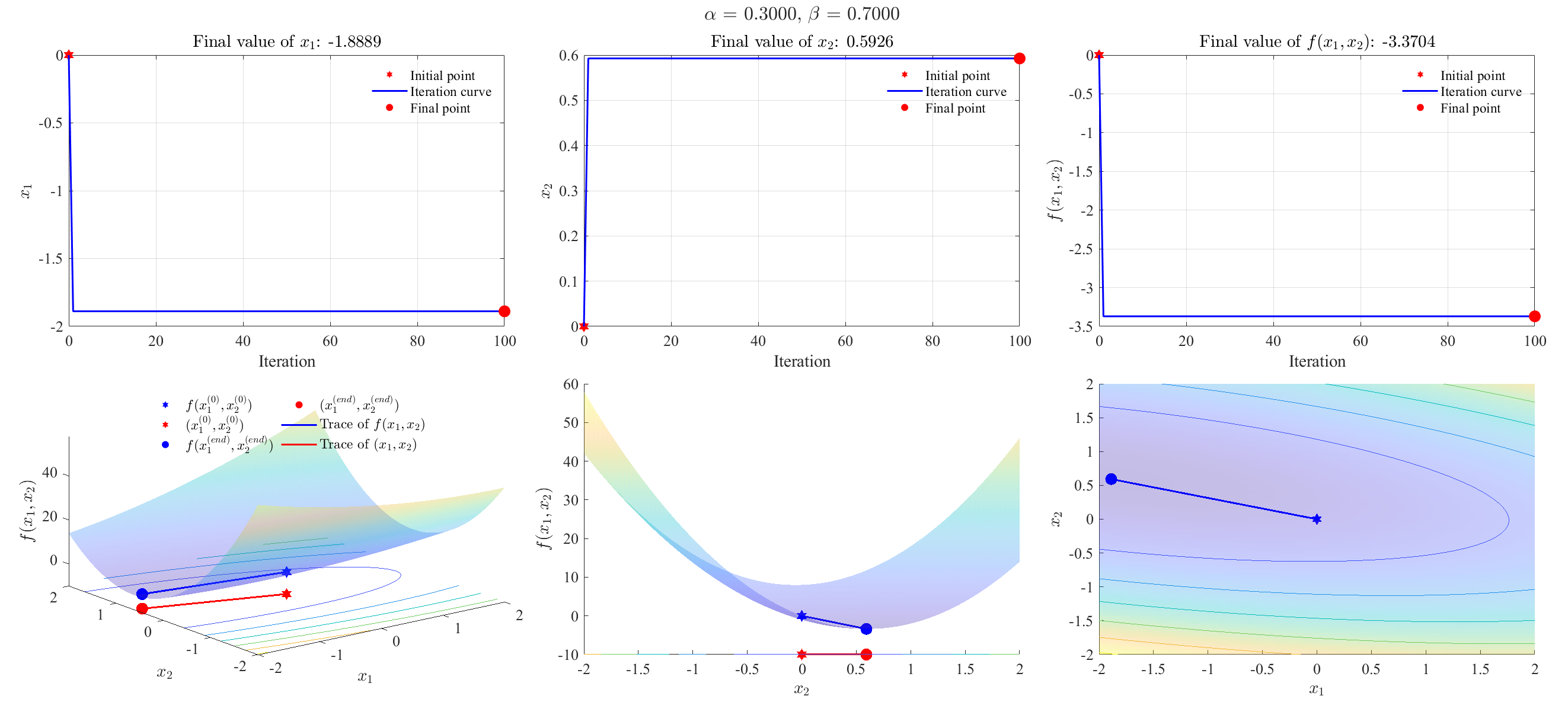
Newton’s method with backtracking line-search
Set $\alpha=0.3$ in Eq. $\eqref{eq2}$, and $\beta = 0.7$ in Eq. $\eqref{eq4}$.
1
2
3
4
5
6
7
8
9
10
11
12
13
14
15
16
17
18
19
20
21
22
23
24
25
26
27
28
29
30
31
32
33
34
35
36
37
38
39
40
41
42
43
44
45
46
47
48
49
50
51
52
53
54
55
56
57
58
59
60
61
62
63
64
65
66
67
68
69
70
71
72
73
74
75
76
77
78
79
80
81
82
83
84
85
86
87
88
89
90
91
92
93
94
95
96
97
98
99
100
101
102
103
104
105
106
107
108
109
110
111
112
113
114
115
116
117
118
119
120
121
122
123
124
125
126
127
128
129
130
131
132
133
134
135
136
137
138
139
140
141
142
143
144
145
146
147
148
149
150
151
152
153
154
155
156
157
158
159
160
161
162
163
164
165
166
167
168
169
170
171
172
173
174
175
176
177
178
179
180
181
182
183
184
185
186
187
188
189
190
191
192
193
194
195
clc, clear, close all

syms x1 x2
f_sym = x1.^2+3*x1.*x2+9*x2.^2+2*x1-5*x2;

g_sym = gradient(f_sym, [x1, x2]);
H_sym = hessian(f_sym, [x1, x2]);

f = matlabFunction(f_sym, 'Vars', {x1, x2});
g = matlabFunction(g_sym, 'Vars', {x1, x2});
H = matlabFunction(H_sym, 'Vars', {x1, x2});

x0 = [0, 0]';
alpha = 0.3;
beta = 0.7;
helperNewtonwithLineSearch(f, g, H, x0, alpha, beta)

function helperNewtonwithLineSearch(f, g, H, x0, alpha, beta)
xOld = x0;
numIter = 100;

xk = nan(numIter, 2);
iters = (1:numIter)';
for i = 1:numIter
    % ============ Newton's method with backtracking line-search ============
    gi = g(xOld(1), xOld(2));
    Hi = H(xOld(1), xOld(2));

    di = -Hi\gi;

    gamma = 1;
    xNew = xOld+gamma*di;
    fOld = f(xOld(1), xOld(2));

    while f(xNew(1), xNew(2)) >  fOld + gamma*alpha*(gi'*di)
        fprintf("gamma*alpha*(gi'*di): %.4f\n", gamma*alpha*(gi'*di))
        gamma = beta*gamma;
        if gamma < 1e-9
            warning('Line search failed (gamma too small).')
            break
        end
        xNew = xOld+gamma*di;
    end
    % ====================================

    xk(i,:) = xNew;
    xOld = xNew;

    % % Stop if diverge
    % if f(xNew(1), xNew(2))>100
    %     break
    % end
    %
    % % Early stop if converge
    % if i>1 && norm(f(xk(i,1), xk(i,2)) - f(xk(i-1,1), xk(i-1,2)))<=1e-4
    %     xk(i+1:end, :) = [];
    %     iters(i+1:end) = [];
    %     break
    % end
end

xk(isnan(xk)) = [];

xs1 = [x0(1); xk(:,1)];
xs2 = [x0(2); xk(:,2)];
iters = [0; iters(1:(height(xs1)-1))];
fs = f(xs1, xs2);

fprintf('Final function value: %.4f\n', f(xNew(1), xNew(2)))

% Present results
helperPlot(f, xs1, xs2, iters, fs, alpha, beta)
end

function helperPlot(f, xs1, xs2, iters, fs, alpha, beta)
figure('Color', 'w', 'Position', [305,283,1915,835])
tiledlayout(2, 3, 'TileSpacing', 'compact')
LineWidth = 1.5;
FontSize = 13;
FontName = 'Times New Roman';

%% Axes 1
nexttile
hold(gca, 'on'), grid(gca, 'on'), box(gca, 'on')
scatter(iters(1), xs1(1), 100, 'Marker', 'hexagram', ...
    'MarkerFaceColor', 'r', 'MarkerEdgeColor', 'none', 'DisplayName', 'Initial point')
plot(iters, xs1, 'LineWidth', LineWidth, 'Color', 'b', 'DisplayName', 'Iteration curve')
scatter(iters(end), xs1(end), 100, 'Marker', 'o', ...
    'MarkerFaceColor', 'r', 'MarkerEdgeColor', 'none', 'DisplayName', 'Final point')
xlabel('Iteration')
ylabel('$x_1$', 'Interpreter', 'latex')
legend('Box', 'off')
title(sprintf('Final value of %s: %.4f', '$x_1$', xs1(end)), 'Interpreter', 'latex')
set(gca, 'FontSize', FontSize, 'FontName', FontName)

%% Axes 2
nexttile
hold(gca, 'on'), grid(gca, 'on'), box(gca, 'on')
scatter(iters(1), xs2(1), 100, 'Marker', 'hexagram', ...
    'MarkerFaceColor', 'r', 'MarkerEdgeColor', 'none', 'DisplayName', 'Initial point')
plot(iters, xs2, 'LineWidth', LineWidth, 'Color', 'b', 'DisplayName', 'Iteration curve')
scatter(iters(end), xs2(end), 100, 'Marker', 'o', ...
    'MarkerFaceColor', 'r', 'MarkerEdgeColor', 'none', 'DisplayName', 'Final point')
xlabel('Iteration')
ylabel('$x_2$', 'Interpreter', 'latex')
legend('Box', 'off')
title(sprintf('Final value of %s: %.4f', '$x_2$', xs2(end)), 'Interpreter', 'latex')
set(gca, 'FontSize', FontSize, 'FontName', FontName)

%% Axes 3
nexttile
hold(gca, 'on'), grid(gca, 'on'), box(gca, 'on')
scatter(iters(1), fs(1), 100, 'Marker', 'hexagram', ...
    'MarkerFaceColor', 'r', 'MarkerEdgeColor', 'none', 'DisplayName', 'Initial point')
plot(iters, fs, 'LineWidth', LineWidth, 'Color', 'b', 'DisplayName', 'Iteration curve')
scatter(iters(end), fs(end), 100, 'Marker', 'o', ...
    'MarkerFaceColor', 'r', 'MarkerEdgeColor', 'none', 'DisplayName', 'Final point')
xlabel('Iteration')
ylabel('$f(x_1,x_2)$', 'Interpreter', 'latex')
legend('Box', 'off')
title(sprintf('Final value of %s: %.4f', '$f(x_1,x_2)$', fs(end)), 'Interpreter', 'latex')
set(gca, 'FontSize', FontSize, 'FontName', FontName)

%% Axes 4
nexttile
view(3)
hold(gca, 'on')
ax1 = gca();

x_min = -2;
x_max = 2;
x1 = linspace(x_min, x_max, 100);
x2 = linspace(x_min, x_max, 100);

[X1, X2] = meshgrid(x1, x2);
y = f(X1, X2);
sc = surfc(X1, X2, y, 'FaceAlpha', 0.3, 'EdgeColor', 'none', 'DisplayName', '$f(x_1,x_2)$', 'HandleVisibility', 'off');
sc(2).HandleVisibility = 'off';
sc(2).LevelList = min(y,[],"all"):10:max(y,[],"all");
LevelStep = sc(2).LevelStep;

scatter3(xs1(1), xs2(1), fs(1), 100, 'Marker', 'hexagram', ...
    'MarkerFaceColor', 'b', 'MarkerEdgeColor', 'none', 'DisplayName', '$f(x_1^{(0)}, x_2^{(0)})$')
scatter3(xs1(1), xs2(1), -LevelStep, 100, 'Marker', 'hexagram', ...
    'MarkerFaceColor', 'r', 'MarkerEdgeColor', 'none', 'DisplayName', '$(x_1^{(0)}, x_2^{(0)})$')
scatter3(xs1(end), xs2(end), fs(end), 100, 'Marker', 'o', ...
    'MarkerFaceColor', 'b', 'MarkerEdgeColor', 'none', 'DisplayName', '$f(x_1^{(end)}, x_2^{(end)})$')
scatter3(xs1(end), xs2(end), -LevelStep, 100, 'Marker', 'o', ...
    'MarkerFaceColor', 'r', 'MarkerEdgeColor', 'none', 'DisplayName', '$(x_1^{(end)}, x_2^{(end)})$')

plot3(xs1, xs2, fs, 'LineWidth', LineWidth, 'Color', 'b', 'DisplayName', 'Trace of $f(x_1,x_2)$')
plot3(xs1, xs2, -LevelStep*ones(size(xs1)), 'LineWidth', LineWidth, 'Color', 'r', 'DisplayName', 'Trace of $(x_1,x_2)$')
% helperFill3(xs1, xs2, fs, xs1, xs2, -LevelStep*ones(size(xs1)), 'g')

xlim([x_min, x_max])
ylim([x_min, x_max])
xlabel('$x_1$', 'Interpreter', 'latex')
ylabel('$x_2$', 'Interpreter', 'latex')
zlabel('$f(x_1,x_2)$', 'Interpreter', 'latex')
lgd1 = legend('Interpreter', 'latex', 'Box', 'off', 'NumColumns', 2, 'Location', 'north', 'EdgeColor', 'none');
set(gca, 'FontSize', FontSize, 'FontName', FontName)

%% Axes 5
nexttile
ax2 = gca();
copyobj(allchild(ax1), ax2);
view([90,0])
xlim([x_min, x_max])
ylim([x_min, x_max])
xlabel('$x_1$', 'Interpreter', 'latex')
ylabel('$x_2$', 'Interpreter', 'latex')
zlabel('$f(x_1,x_2)$', 'Interpreter', 'latex')
% legend(ax2, lgd1.String, 'Interpreter', lgd1.Interpreter, ...
%     'Box', lgd1.Box, 'NumColumns', lgd1.NumColumns, ...
%     'Location', lgd1.Location, 'EdgeColor', lgd1.EdgeColor);
set(ax2, 'FontSize', FontSize, 'FontName', FontName)

%% Axes 6
nexttile
ax3 = gca();
copyobj(allchild(ax1), ax3);
view([0,90])
xlim([x_min, x_max])
ylim([x_min, x_max])
xlabel('$x_1$', 'Interpreter', 'latex')
ylabel('$x_2$', 'Interpreter', 'latex')
zlabel('$f(x_1,x_2)$', 'Interpreter', 'latex')
% legend(ax3, lgd1.String, 'Interpreter', lgd1.Interpreter, ...
%     'Box', lgd1.Box, 'NumColumns', lgd1.NumColumns, ...
%     'Location', lgd1.Location, 'EdgeColor', lgd1.EdgeColor);
set(gca, 'FontSize', FontSize, 'FontName', FontName)

sgtitle(sprintf('%s = %.4f, %s = %.4f', "$\alpha$", alpha, "$\beta$", beta), 'Interpreter', 'latex', ...
    'FontSize', FontSize+3, 'FontName', FontName)
end
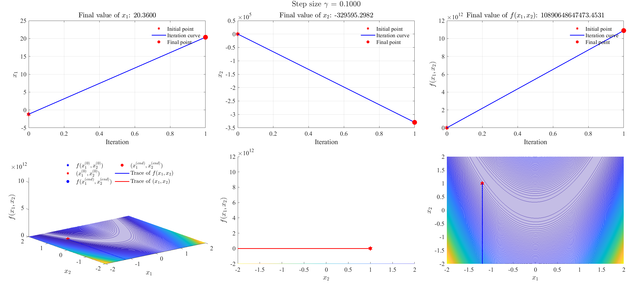
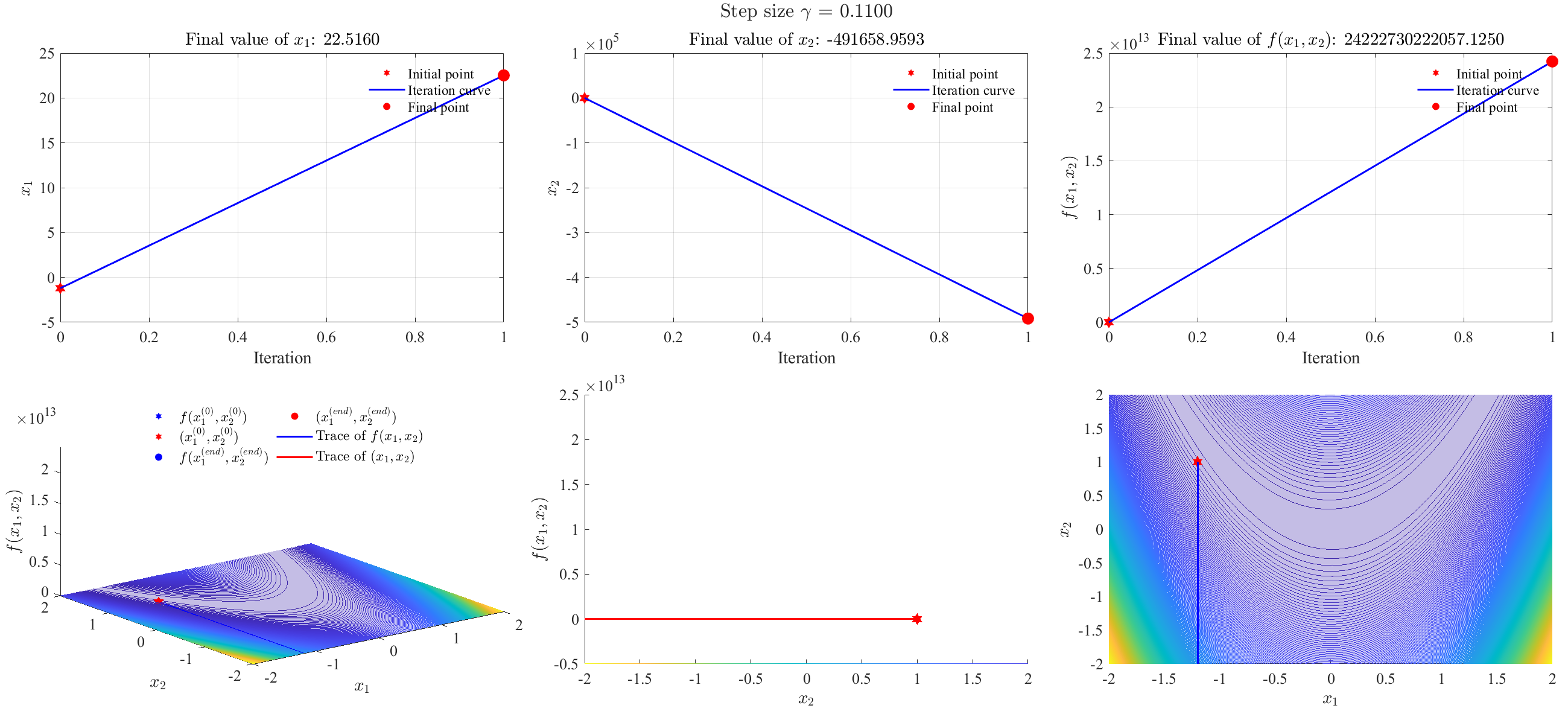
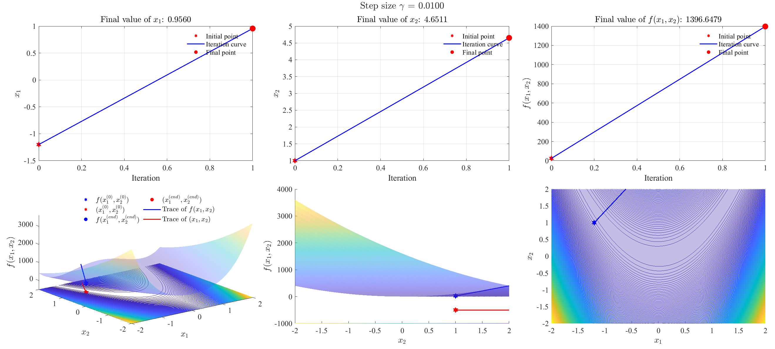
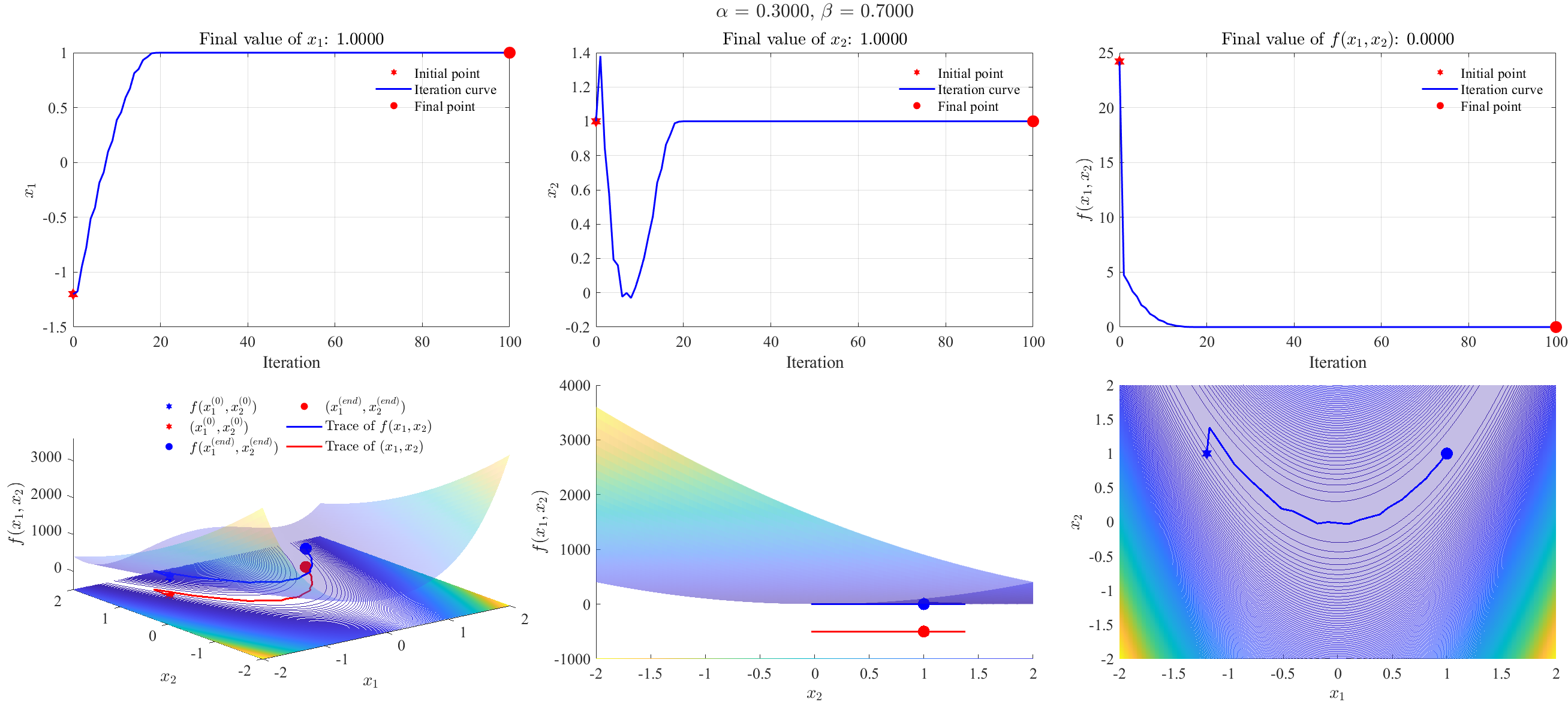
Example 2: Rosenbrock function
Consider a Rosenbrock function7:
\[f(x_1,x_2) = (1-x_1)^2+100(x_2-x_1^2)^2\]Select $\boldsymbol{x}^{(0)} = [-1.2,1]^T$, and maximum iteration is 100.
Gradient descent algorithm (divergent)
Step size = 0.1 (divergent)
Step size = 0.11 (divergent)
Step size = 0.01 (divergent)
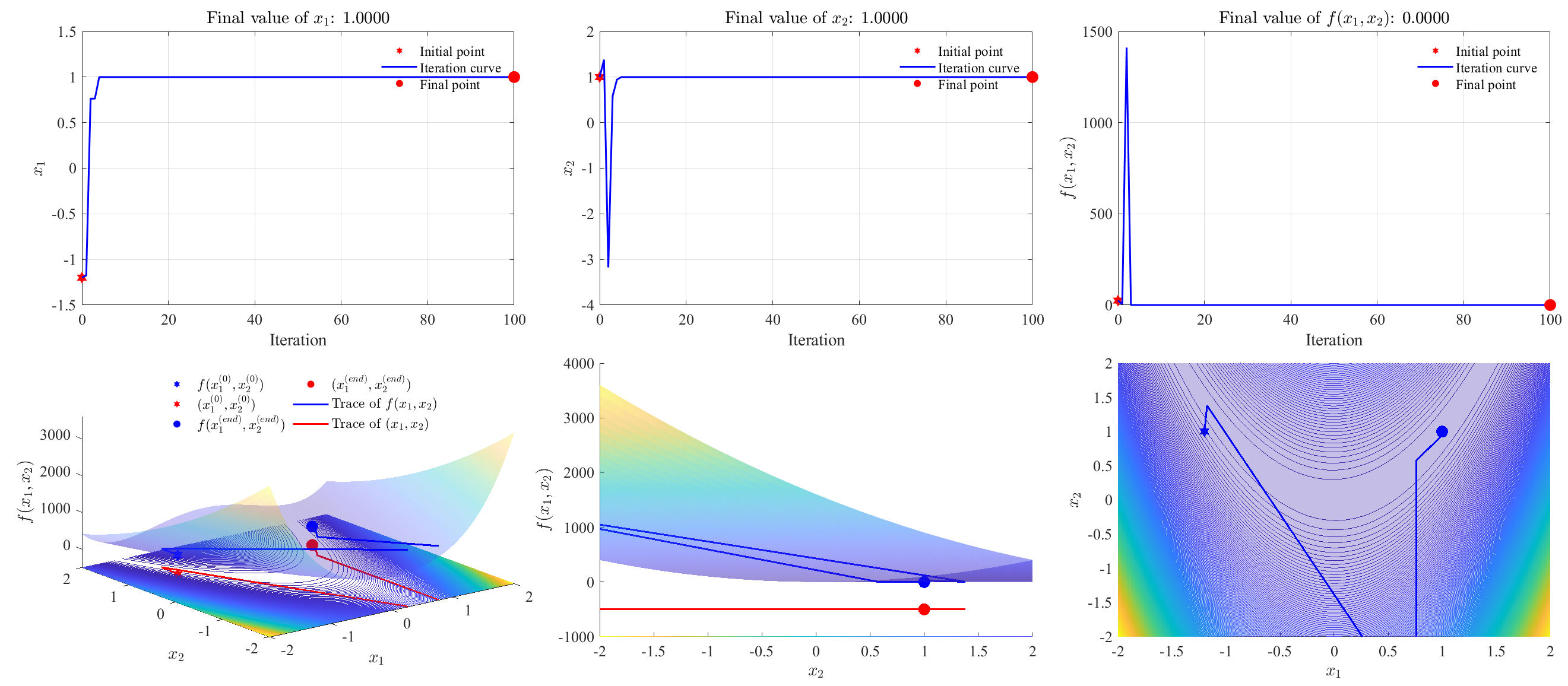
Newton’s method (convergent)
Newton’s method with backtracking line-search (convergent)
Again, set $\alpha=0.3$ in Eq. $\eqref{eq2}$, and $\beta = 0.7$ in Eq. $\eqref{eq4}$.
1
2
3
4
5
6
7
8
9
10
11
12
13
14
15
gamma*alpha*(gi'*di): -2.5300
gamma*alpha*(gi'*di): -1.7710
gamma*alpha*(gi'*di): -1.2397
gamma*alpha*(gi'*di): -0.8678
gamma*alpha*(gi'*di): -0.6074
gamma*alpha*(gi'*di): -0.4252
gamma*alpha*(gi'*di): -0.3999
gamma*alpha*(gi'*di): -0.2799
gamma*alpha*(gi'*di): -0.2569
gamma*alpha*(gi'*di): -0.1798
gamma*alpha*(gi'*di): -0.1353
gamma*alpha*(gi'*di): -0.0900
gamma*alpha*(gi'*di): -0.0630
gamma*alpha*(gi'*di): -0.0106
Final function value: 0.0000
Brief summary
To conclude:
- For above two test cases, Newton’s method with backtracking line-search behaves the best, leading to convergent results, and the gradient descent the worst, relying much on the choice of step size.
- As for parameters,
- Gradient descent: need to specify a (1) step size;
- Newton’s method: no parameter should be specified;
- Newton’s method with backtracking line-search: need to specify two parameters, (1) $\alpha$ in Eq. $\eqref{eq2}$, and (2) $\beta$ in Eq. $\eqref{eq4}$.
The minimum code
In above MATLAB script, the minimum code to realize three algorithms shows as follows.
Gradient descent
1
2
3
4
5
6
7
8
9
10
11
12
13
14
15
16
17
18
19
20
21
22
23
24
25
26
27
28
29
30
31
32
33
34
35
36
37
38
function helperGD(f, g, gamma, x0)
xOld = x0;
numIter = 100;

xk = nan(numIter, 2);
iters = (1:numIter)';

for i = 1:numIter
    % ============ Gradient descent ============
    gi = g(xOld(1), xOld(2));
    xNew = xOld-gamma*gi;
    % ====================================

    xk(i,:) = xNew;
    xOld = xNew;

    % % Stop if diverge
    % if f(xNew(1), xNew(2))>1e5
    %     break
    % end

    % % Early stop if converge
    % if i>1 && norm(f(xk(i,1), xk(i,2)) - f(xk(i-1,1), xk(i-1,2)))<=1e-4
    %     xk(i+1:end, :) = [];
    %     iters(i+1:end) = [];
    %     break
    % end
end

xk(isnan(xk)) = [];

xs1 = [x0(1); xk(:,1)];
xs2 = [x0(2); xk(:,2)];
iters = [0; iters(1:(height(xs1)-1))];
fs = f(xs1, xs2);

fprintf('Final function value: %.4f\n', f(xNew(1), xNew(2)))
end
Newton’s method
1
2
3
4
5
6
7
8
9
10
11
12
13
14
15
16
17
18
19
20
21
22
23
24
25
26
27
28
29
30
31
32
33
34
35
36
37
38
39
40
function helperNewton(f, g, H, x0)
xOld = x0;
numIter = 100;

xk = nan(numIter, 2);
iters = (1:numIter)';

for i = 1:numIter
    %  ============ Newton's method ============
    gi = g(xOld(1), xOld(2));
    Hi = H(xOld(1), xOld(2));

    xNew = xOld-Hi\gi;
    % =====================================

    xk(i,:) = xNew;
    xOld = xNew;

    % % Stop if diverge
    % if f(xNew(1), xNew(2))>100
    %     break
    % end
    %
    % % Early stop if converge
    % if i>1 && norm(f(xk(i,1), xk(i,2)) - f(xk(i-1,1), xk(i-1,2)))<=1e-4
    %     xk(i+1:end, :) = [];
    %     iters(i+1:end) = [];
    %     break
    % end
end

xk(isnan(xk)) = [];

xs1 = [x0(1); xk(:,1)];
xs2 = [x0(2); xk(:,2)];
iters = [0; iters(1:(height(xs1)-1))];
fs = f(xs1, xs2);

fprintf('Final function value: %.4f\n', f(xNew(1), xNew(2)))
end
Newton’s method with backtracking line-search
1
2
3
4
5
6
7
8
9
10
11
12
13
14
15
16
17
18
19
20
21
22
23
24
25
26
27
28
29
30
31
32
33
34
35
36
37
38
39
40
41
42
43
44
45
46
47
48
49
50
51
52
53
function helperNewtonwithLineSearch(f, g, H, x0, alpha, beta)
xOld = x0;
numIter = 100;

xk = nan(numIter, 2);
iters = (1:numIter)';
for i = 1:numIter
    % ============ Newton's method with backtracking line-search ============
    gi = g(xOld(1), xOld(2));
    Hi = H(xOld(1), xOld(2));

    di = -Hi\gi;

    gamma = 1;
    xNew = xOld+gamma*di;
    fOld = f(xOld(1), xOld(2));

    while f(xNew(1), xNew(2)) >  fOld + gamma*alpha*(gi'*di)
        fprintf("gamma*alpha*(gi'*di): %.4f\n", gamma*alpha*(gi'*di))
        gamma = beta*gamma;
        if gamma < 1e-9
            warning('Line search failed (gamma too small).')
            break
        end
        xNew = xOld+gamma*di;
    end
    % ====================================

    xk(i,:) = xNew;
    xOld = xNew;

    % % Stop if diverge
    % if f(xNew(1), xNew(2))>100
    %     break
    % end
    %
    % % Early stop if converge
    % if i>1 && norm(f(xk(i,1), xk(i,2)) - f(xk(i-1,1), xk(i-1,2)))<=1e-4
    %     xk(i+1:end, :) = [];
    %     iters(i+1:end) = [];
    %     break
    % end
end

xk(isnan(xk)) = [];

xs1 = [x0(1); xk(:,1)];
xs2 = [x0(2); xk(:,2)];
iters = [0; iters(1:(height(xs1)-1))];
fs = f(xs1, xs2);

fprintf('Final function value: %.4f\n', f(xNew(1), xNew(2)))
end
References
-
Review Notes and Supplementary Notes CS229 Course Machine Learning Standford University, Convex Optimization Overview (cnt’d), pp. 8-9. ˄ ˄2
-
Solve Non-linear Equation and Equations System by Iterative Methods — Bisection Method, Fixed Point Iteration, Newton’s Method, Secant Method, Multivariate Newton’s Method, and Broyden’s Method. ˄
-
A Simple Gradient Descend (GD) and A Stochastic Gradient Descend (SGD) to Select Optimum Weight of Linear Model. ˄